7 Traversing Graphs
\(\newcommand{\footnotename}{footnote}\)
\(\def \LWRfootnote {1}\)
\(\newcommand {\footnote }[2][\LWRfootnote ]{{}^{\mathrm {#1}}}\)
\(\newcommand {\footnotemark }[1][\LWRfootnote ]{{}^{\mathrm {#1}}}\)
\(\let \LWRorighspace \hspace \)
\(\renewcommand {\hspace }{\ifstar \LWRorighspace \LWRorighspace }\)
\(\newcommand {\TextOrMath }[2]{#2}\)
\(\newcommand {\mathnormal }[1]{{#1}}\)
\(\newcommand \ensuremath [1]{#1}\)
\(\newcommand {\LWRframebox }[2][]{\fbox {#2}} \newcommand {\framebox }[1][]{\LWRframebox } \)
\(\newcommand {\setlength }[2]{}\)
\(\newcommand {\addtolength }[2]{}\)
\(\newcommand {\setcounter }[2]{}\)
\(\newcommand {\addtocounter }[2]{}\)
\(\newcommand {\arabic }[1]{}\)
\(\newcommand {\number }[1]{}\)
\(\newcommand {\noalign }[1]{\text {#1}\notag \\}\)
\(\newcommand {\cline }[1]{}\)
\(\newcommand {\directlua }[1]{\text {(directlua)}}\)
\(\newcommand {\luatexdirectlua }[1]{\text {(directlua)}}\)
\(\newcommand {\protect }{}\)
\(\def \LWRabsorbnumber #1 {}\)
\(\def \LWRabsorbquotenumber "#1 {}\)
\(\newcommand {\LWRabsorboption }[1][]{}\)
\(\newcommand {\LWRabsorbtwooptions }[1][]{\LWRabsorboption }\)
\(\def \mathchar {\ifnextchar "\LWRabsorbquotenumber \LWRabsorbnumber }\)
\(\def \mathcode #1={\mathchar }\)
\(\let \delcode \mathcode \)
\(\let \delimiter \mathchar \)
\(\def \oe {\unicode {x0153}}\)
\(\def \OE {\unicode {x0152}}\)
\(\def \ae {\unicode {x00E6}}\)
\(\def \AE {\unicode {x00C6}}\)
\(\def \aa {\unicode {x00E5}}\)
\(\def \AA {\unicode {x00C5}}\)
\(\def \o {\unicode {x00F8}}\)
\(\def \O {\unicode {x00D8}}\)
\(\def \l {\unicode {x0142}}\)
\(\def \L {\unicode {x0141}}\)
\(\def \ss {\unicode {x00DF}}\)
\(\def \SS {\unicode {x1E9E}}\)
\(\def \dag {\unicode {x2020}}\)
\(\def \ddag {\unicode {x2021}}\)
\(\def \P {\unicode {x00B6}}\)
\(\def \copyright {\unicode {x00A9}}\)
\(\def \pounds {\unicode {x00A3}}\)
\(\let \LWRref \ref \)
\(\renewcommand {\ref }{\ifstar \LWRref \LWRref }\)
\( \newcommand {\multicolumn }[3]{#3}\)
\(\require {textcomp}\)
\(\newcommand {\intertext }[1]{\text {#1}\notag \\}\)
\(\let \Hat \hat \)
\(\let \Check \check \)
\(\let \Tilde \tilde \)
\(\let \Acute \acute \)
\(\let \Grave \grave \)
\(\let \Dot \dot \)
\(\let \Ddot \ddot \)
\(\let \Breve \breve \)
\(\let \Bar \bar \)
\(\let \Vec \vec \)
\(\renewcommand {\vec }{\boldsymbol }\)
\(\newcommand {\Edge }{\ensuremath {\,\textemdash \,}}\)
\(\newcommand \Const [1]{\text {\textsf {#1}}}\)
\(\DeclareMathOperator {\lerp }{lerp}\)
\(\DeclareMathOperator {\bitlen }{bitlen}\)
\(\DeclareMathOperator {\sign }{sign}\)
\(\newcommand {\I }{\mathrm {i}}\)
\(\newcommand \AND {\mathbin {\&}}\)
\(\newcommand \OR {\mathbin {|}}\)
\(\newcommand \XOR {\mathbin {{}^{\wedge }}}\)
\(\newcommand \shl {\ll }\)
\(\newcommand \shr {\ggg }\)
\(\newcommand \asr {\gg }\)
\(\newcommand \NOT {\ensuremath {\mathord {\sim }}}\)
\(\newcommand {\isep }{\mathrel {{.}\,{.}}}\)
\(\newcommand {\Id }[1]{\mathit {#1}}\)
\(\newcommand {\const }[1]{\mathsf {#1}}\)
\(\newcommand {\algorithmname }[1]{\text {\textsc {#1}}}\)
\(\newcommand {\bits }[1]{\text {#1}}\)
\(\newcommand {\hexa }[1]{\mathtt {0x#1}}\)
\(\newcommand {\num }[1]{#1}\)
\(\newcommand {\qed }{\quad \square }\)
\(\newcommand {\idiv }[2]{\lfloor #1/#2\rfloor }\)
\(\newcommand \attribdot {\ensuremath {\mkern 1.5mu.\mkern 1.5mu}}\)
\(\newcommand \attribxr [2]{#1\attribdot \text {#2}}\)
\(\newcommand \attribir [2]{\Id {#1}\attribdot \text {#2}}\)
\(\newcommand \attribii [2]{\Id {#1}\attribdot \Id {#2}}\)
\(\newcommand \textsc [1]{#1}\)
\(\require {colortbl}\)
\(\let \LWRorigcolumncolor \columncolor \)
\(\renewcommand {\columncolor }[2][named]{\LWRorigcolumncolor [#1]{#2}\LWRabsorbtwooptions }\)
\(\let \LWRorigrowcolor \rowcolor \)
\(\renewcommand {\rowcolor }[2][named]{\LWRorigrowcolor [#1]{#2}\LWRabsorbtwooptions }\)
\(\let \LWRorigcellcolor \cellcolor \)
\(\renewcommand {\cellcolor }[2][named]{\LWRorigcellcolor [#1]{#2}\LWRabsorbtwooptions }\)
\(\newcommand {\tcbset }[1]{}\)
\(\newcommand {\tcbsetforeverylayer }[1]{}\)
\(\newcommand {\tcbox }[2][]{\boxed {\text {#2}}}\)
\(\newcommand {\tcboxfit }[2][]{\boxed {#2}}\)
\(\newcommand {\tcblower }{}\)
\(\newcommand {\tcbline }{}\)
\(\newcommand {\tcbtitle }{}\)
\(\newcommand {\tcbsubtitle [2][]{\mathrm {#2}}}\)
\(\newcommand {\tcboxmath }[2][]{\boxed {#2}}\)
\(\newcommand {\tcbhighmath }[2][]{\boxed {#2}}\)
\(\newcommand {\toprule }[1][]{\hline }\)
\(\let \midrule \toprule \)
\(\let \bottomrule \toprule \)
\(\def \LWRbooktabscmidruleparen (#1)#2{}\)
\(\newcommand {\LWRbooktabscmidrulenoparen }[1]{}\)
\(\newcommand {\cmidrule }[1][]{\ifnextchar (\LWRbooktabscmidruleparen \LWRbooktabscmidrulenoparen }\)
\(\newcommand {\morecmidrules }{}\)
\(\newcommand {\specialrule }[3]{\hline }\)
\(\newcommand {\addlinespace }[1][]{}\)
\(\newcommand {\LWRsubmultirow }[2][]{#2}\)
\(\newcommand {\LWRmultirow }[2][]{\LWRsubmultirow }\)
\(\newcommand {\multirow }[2][]{\LWRmultirow }\)
\(\newcommand {\mrowcell }{}\)
\(\newcommand {\mcolrowcell }{}\)
\(\newcommand {\STneed }[1]{}\)
\(\newcommand {\LWRldelimtwo }[1][]{\text {#1}~\LWRbigdelim }\)
\(\newcommand {\LWRldelimone }[2][]{\LWRldelimtwo }\)
\(\def \ldelim #1#2{\def \LWRbigdelim {#1}\LWRldelimone }\)
\(\newcommand {\LWRrdelimtwo }[1][]{\LWRbigdelim ~\text {#1}}\)
\(\newcommand {\LWRrdelimone }[2][]{\LWRrdelimtwo }\)
\(\def \rdelim #1#2{\def \LWRbigdelim {#1}\LWRrdelimone }\)
\(\let \symnormal \mathit \)
\(\let \symliteral \mathrm \)
\(\let \symbb \mathbb \)
\(\let \symbbit \mathbb \)
\(\let \symcal \mathcal \)
\(\let \symscr \mathscr \)
\(\let \symfrak \mathfrak \)
\(\let \symsfup \mathsf \)
\(\let \symsfit \mathit \)
\(\let \symbfsf \mathbf \)
\(\let \symbfup \mathbf \)
\(\newcommand {\symbfit }[1]{\boldsymbol {#1}}\)
\(\let \symbfcal \mathcal \)
\(\let \symbfscr \mathscr \)
\(\let \symbffrak \mathfrak \)
\(\let \symbfsfup \mathbf \)
\(\newcommand {\symbfsfit }[1]{\boldsymbol {#1}}\)
\(\let \symup \mathrm \)
\(\let \symbf \mathbf \)
\(\let \symit \mathit \)
\(\let \symsf \symsfit \)
\(\let \symtt \mathtt \)
\(\let \symbffrac \mathbffrac \)
\(\newcommand {\mathfence }[1]{\mathord {#1}}\)
\(\newcommand {\mathover }[1]{#1}\)
\(\newcommand {\mathunder }[1]{#1}\)
\(\newcommand {\mathaccent }[1]{#1}\)
\(\newcommand {\mathbotaccent }[1]{#1}\)
\(\newcommand {\mathalpha }[1]{\mathord {#1}}\)
\(\def\Alpha{\unicode{x1D6E2}}\)
\(\def\Beta{\unicode{x1D6E3}}\)
\(\def\Gamma{\unicode{x1D6E4}}\)
\(\def\Digamma{\mathit{\unicode{x03DC}}}\)
\(\def\Delta{\unicode{x1D6E5}}\)
\(\def\Epsilon{\unicode{x1D6E6}}\)
\(\def\Zeta{\unicode{x1D6E7}}\)
\(\def\Eta{\unicode{x1D6E8}}\)
\(\def\Theta{\unicode{x1D6E9}}\)
\(\def\Vartheta{\unicode{x1D6F3}}\)
\(\def\Iota{\unicode{x1D6EA}}\)
\(\def\Kappa{\unicode{x1D6EB}}\)
\(\def\Lambda{\unicode{x1D6EC}}\)
\(\def\Mu{\unicode{x1D6ED}}\)
\(\def\Nu{\unicode{x1D6EE}}\)
\(\def\Xi{\unicode{x1D6EF}}\)
\(\def\Omicron{\unicode{x1D6F0}}\)
\(\def\Pi{\unicode{x1D6F1}}\)
\(\def\Rho{\unicode{x1D6F2}}\)
\(\def\Sigma{\unicode{x1D6F4}}\)
\(\def\Tau{\unicode{x1D6F5}}\)
\(\def\Upsilon{\unicode{x1D6F6}}\)
\(\def\Phi{\unicode{x1D6F7}}\)
\(\def\Chi{\unicode{x1D6F8}}\)
\(\def\Psi{\unicode{x1D6F9}}\)
\(\def\Omega{\unicode{x1D6FA}}\)
\(\def\alpha{\unicode{x1D6FC}}\)
\(\def\beta{\unicode{x1D6FD}}\)
\(\def\varbeta{\unicode{x03D0}}\)
\(\def\gamma{\unicode{x1D6FE}}\)
\(\def\digamma{\mathit{\unicode{x03DD}}}\)
\(\def\delta{\unicode{x1D6FF}}\)
\(\def\epsilon{\unicode{x1D716}}\)
\(\def\varepsilon{\unicode{x1D700}}\)
\(\def\zeta{\unicode{x1D701}}\)
\(\def\eta{\unicode{x1D702}}\)
\(\def\theta{\unicode{x1D703}}\)
\(\def\vartheta{\unicode{x1D717}}\)
\(\def\iota{\unicode{x1D704}}\)
\(\def\kappa{\unicode{x1D705}}\)
\(\def\varkappa{\unicode{x1D718}}\)
\(\def\lambda{\unicode{x1D706}}\)
\(\def\mu{\unicode{x1D707}}\)
\(\def\nu{\unicode{x1D708}}\)
\(\def\xi{\unicode{x1D709}}\)
\(\def\omicron{\unicode{x1D70A}}\)
\(\def\pi{\unicode{x1D70B}}\)
\(\def\varpi{\unicode{x1D71B}}\)
\(\def\rho{\unicode{x1D70C}}\)
\(\def\varrho{\unicode{x1D71A}}\)
\(\def\sigma{\unicode{x1D70E}}\)
\(\def\varsigma{\unicode{x1D70D}}\)
\(\def\tau{\unicode{x1D70F}}\)
\(\def\upsilon{\unicode{x1D710}}\)
\(\def\phi{\unicode{x1D719}}\)
\(\def\varphi{\unicode{x1D711}}\)
\(\def\chi{\unicode{x1D712}}\)
\(\def\psi{\unicode{x1D713}}\)
\(\def\omega{\unicode{x1D714}}\)
\(\def\upAlpha{\unicode{x0391}}\)
\(\def\upBeta{\unicode{x0392}}\)
\(\def\upGamma{\unicode{x0393}}\)
\(\def\upDigamma{\unicode{x03DC}}\)
\(\def\upDelta{\unicode{x0394}}\)
\(\def\upEpsilon{\unicode{x0395}}\)
\(\def\upZeta{\unicode{x0396}}\)
\(\def\upEta{\unicode{x0397}}\)
\(\def\upTheta{\unicode{x0398}}\)
\(\def\upVartheta{\unicode{x03F4}}\)
\(\def\upIota{\unicode{x0399}}\)
\(\def\upKappa{\unicode{x039A}}\)
\(\def\upLambda{\unicode{x039B}}\)
\(\def\upMu{\unicode{x039C}}\)
\(\def\upNu{\unicode{x039D}}\)
\(\def\upXi{\unicode{x039E}}\)
\(\def\upOmicron{\unicode{x039F}}\)
\(\def\upPi{\unicode{x03A0}}\)
\(\def\upVarpi{\unicode{x03D6}}\)
\(\def\upRho{\unicode{x03A1}}\)
\(\def\upSigma{\unicode{x03A3}}\)
\(\def\upTau{\unicode{x03A4}}\)
\(\def\upUpsilon{\unicode{x03A5}}\)
\(\def\upPhi{\unicode{x03A6}}\)
\(\def\upChi{\unicode{x03A7}}\)
\(\def\upPsi{\unicode{x03A8}}\)
\(\def\upOmega{\unicode{x03A9}}\)
\(\def\itAlpha{\unicode{x1D6E2}}\)
\(\def\itBeta{\unicode{x1D6E3}}\)
\(\def\itGamma{\unicode{x1D6E4}}\)
\(\def\itDigamma{\mathit{\unicode{x03DC}}}\)
\(\def\itDelta{\unicode{x1D6E5}}\)
\(\def\itEpsilon{\unicode{x1D6E6}}\)
\(\def\itZeta{\unicode{x1D6E7}}\)
\(\def\itEta{\unicode{x1D6E8}}\)
\(\def\itTheta{\unicode{x1D6E9}}\)
\(\def\itVartheta{\unicode{x1D6F3}}\)
\(\def\itIota{\unicode{x1D6EA}}\)
\(\def\itKappa{\unicode{x1D6EB}}\)
\(\def\itLambda{\unicode{x1D6EC}}\)
\(\def\itMu{\unicode{x1D6ED}}\)
\(\def\itNu{\unicode{x1D6EE}}\)
\(\def\itXi{\unicode{x1D6EF}}\)
\(\def\itOmicron{\unicode{x1D6F0}}\)
\(\def\itPi{\unicode{x1D6F1}}\)
\(\def\itRho{\unicode{x1D6F2}}\)
\(\def\itSigma{\unicode{x1D6F4}}\)
\(\def\itTau{\unicode{x1D6F5}}\)
\(\def\itUpsilon{\unicode{x1D6F6}}\)
\(\def\itPhi{\unicode{x1D6F7}}\)
\(\def\itChi{\unicode{x1D6F8}}\)
\(\def\itPsi{\unicode{x1D6F9}}\)
\(\def\itOmega{\unicode{x1D6FA}}\)
\(\def\upalpha{\unicode{x03B1}}\)
\(\def\upbeta{\unicode{x03B2}}\)
\(\def\upvarbeta{\unicode{x03D0}}\)
\(\def\upgamma{\unicode{x03B3}}\)
\(\def\updigamma{\unicode{x03DD}}\)
\(\def\updelta{\unicode{x03B4}}\)
\(\def\upepsilon{\unicode{x03F5}}\)
\(\def\upvarepsilon{\unicode{x03B5}}\)
\(\def\upzeta{\unicode{x03B6}}\)
\(\def\upeta{\unicode{x03B7}}\)
\(\def\uptheta{\unicode{x03B8}}\)
\(\def\upvartheta{\unicode{x03D1}}\)
\(\def\upiota{\unicode{x03B9}}\)
\(\def\upkappa{\unicode{x03BA}}\)
\(\def\upvarkappa{\unicode{x03F0}}\)
\(\def\uplambda{\unicode{x03BB}}\)
\(\def\upmu{\unicode{x03BC}}\)
\(\def\upnu{\unicode{x03BD}}\)
\(\def\upxi{\unicode{x03BE}}\)
\(\def\upomicron{\unicode{x03BF}}\)
\(\def\uppi{\unicode{x03C0}}\)
\(\def\upvarpi{\unicode{x03D6}}\)
\(\def\uprho{\unicode{x03C1}}\)
\(\def\upvarrho{\unicode{x03F1}}\)
\(\def\upsigma{\unicode{x03C3}}\)
\(\def\upvarsigma{\unicode{x03C2}}\)
\(\def\uptau{\unicode{x03C4}}\)
\(\def\upupsilon{\unicode{x03C5}}\)
\(\def\upphi{\unicode{x03D5}}\)
\(\def\upvarphi{\unicode{x03C6}}\)
\(\def\upchi{\unicode{x03C7}}\)
\(\def\uppsi{\unicode{x03C8}}\)
\(\def\upomega{\unicode{x03C9}}\)
\(\def\italpha{\unicode{x1D6FC}}\)
\(\def\itbeta{\unicode{x1D6FD}}\)
\(\def\itvarbeta{\unicode{x03D0}}\)
\(\def\itgamma{\unicode{x1D6FE}}\)
\(\def\itdigamma{\mathit{\unicode{x03DD}}}\)
\(\def\itdelta{\unicode{x1D6FF}}\)
\(\def\itepsilon{\unicode{x1D716}}\)
\(\def\itvarepsilon{\unicode{x1D700}}\)
\(\def\itzeta{\unicode{x1D701}}\)
\(\def\iteta{\unicode{x1D702}}\)
\(\def\ittheta{\unicode{x1D703}}\)
\(\def\itvartheta{\unicode{x1D717}}\)
\(\def\itiota{\unicode{x1D704}}\)
\(\def\itkappa{\unicode{x1D705}}\)
\(\def\itvarkappa{\unicode{x1D718}}\)
\(\def\itlambda{\unicode{x1D706}}\)
\(\def\itmu{\unicode{x1D707}}\)
\(\def\itnu{\unicode{x1D708}}\)
\(\def\itxi{\unicode{x1D709}}\)
\(\def\itomicron{\unicode{x1D70A}}\)
\(\def\itpi{\unicode{x1D70B}}\)
\(\def\itvarpi{\unicode{x1D71B}}\)
\(\def\itrho{\unicode{x1D70C}}\)
\(\def\itvarrho{\unicode{x1D71A}}\)
\(\def\itsigma{\unicode{x1D70E}}\)
\(\def\itvarsigma{\unicode{x1D70D}}\)
\(\def\ittau{\unicode{x1D70F}}\)
\(\def\itupsilon{\unicode{x1D710}}\)
\(\def\itphi{\unicode{x1D719}}\)
\(\def\itvarphi{\unicode{x1D711}}\)
\(\def\itchi{\unicode{x1D712}}\)
\(\def\itpsi{\unicode{x1D713}}\)
\(\def\itomega{\unicode{x1D714}}\)
\(\let \lparen (\)
\(\let \rparen )\)
\(\newcommand {\cuberoot }[1]{\,{}^3\!\!\sqrt {#1}}\,\)
\(\newcommand {\fourthroot }[1]{\,{}^4\!\!\sqrt {#1}}\,\)
\(\newcommand {\longdivision }[1]{\mathord {\unicode {x027CC}#1}}\)
\(\newcommand {\mathcomma }{,}\)
\(\newcommand {\mathcolon }{:}\)
\(\newcommand {\mathsemicolon }{;}\)
\(\newcommand {\overbracket }[1]{\mathinner {\overline {\ulcorner {#1}\urcorner }}}\)
\(\newcommand {\underbracket }[1]{\mathinner {\underline {\llcorner {#1}\lrcorner }}}\)
\(\newcommand {\overbar }[1]{\mathord {#1\unicode {x00305}}}\)
\(\newcommand {\ovhook }[1]{\mathord {#1\unicode {x00309}}}\)
\(\newcommand {\ocirc }[1]{\mathord {#1\unicode {x0030A}}}\)
\(\newcommand {\candra }[1]{\mathord {#1\unicode {x00310}}}\)
\(\newcommand {\oturnedcomma }[1]{\mathord {#1\unicode {x00312}}}\)
\(\newcommand {\ocommatopright }[1]{\mathord {#1\unicode {x00315}}}\)
\(\newcommand {\droang }[1]{\mathord {#1\unicode {x0031A}}}\)
\(\newcommand {\leftharpoonaccent }[1]{\mathord {#1\unicode {x020D0}}}\)
\(\newcommand {\rightharpoonaccent }[1]{\mathord {#1\unicode {x020D1}}}\)
\(\newcommand {\vertoverlay }[1]{\mathord {#1\unicode {x020D2}}}\)
\(\newcommand {\leftarrowaccent }[1]{\mathord {#1\unicode {x020D0}}}\)
\(\newcommand {\annuity }[1]{\mathord {#1\unicode {x020E7}}}\)
\(\newcommand {\widebridgeabove }[1]{\mathord {#1\unicode {x020E9}}}\)
\(\newcommand {\asteraccent }[1]{\mathord {#1\unicode {x020F0}}}\)
\(\newcommand {\threeunderdot }[1]{\mathord {#1\unicode {x020E8}}}\)
\(\newcommand {\Bbbsum }{\mathop {\unicode {x2140}}\limits }\)
\(\newcommand {\oiint }{\mathop {\unicode {x222F}}\limits }\)
\(\newcommand {\oiiint }{\mathop {\unicode {x2230}}\limits }\)
\(\newcommand {\intclockwise }{\mathop {\unicode {x2231}}\limits }\)
\(\newcommand {\ointclockwise }{\mathop {\unicode {x2232}}\limits }\)
\(\newcommand {\ointctrclockwise }{\mathop {\unicode {x2233}}\limits }\)
\(\newcommand {\varointclockwise }{\mathop {\unicode {x2232}}\limits }\)
\(\newcommand {\leftouterjoin }{\mathop {\unicode {x27D5}}\limits }\)
\(\newcommand {\rightouterjoin }{\mathop {\unicode {x27D6}}\limits }\)
\(\newcommand {\fullouterjoin }{\mathop {\unicode {x27D7}}\limits }\)
\(\newcommand {\bigbot }{\mathop {\unicode {x27D8}}\limits }\)
\(\newcommand {\bigtop }{\mathop {\unicode {x27D9}}\limits }\)
\(\newcommand {\xsol }{\mathop {\unicode {x29F8}}\limits }\)
\(\newcommand {\xbsol }{\mathop {\unicode {x29F9}}\limits }\)
\(\newcommand {\bigcupdot }{\mathop {\unicode {x2A03}}\limits }\)
\(\newcommand {\bigsqcap }{\mathop {\unicode {x2A05}}\limits }\)
\(\newcommand {\conjquant }{\mathop {\unicode {x2A07}}\limits }\)
\(\newcommand {\disjquant }{\mathop {\unicode {x2A08}}\limits }\)
\(\newcommand {\bigtimes }{\mathop {\unicode {x2A09}}\limits }\)
\(\newcommand {\modtwosum }{\mathop {\unicode {x2A0A}}\limits }\)
\(\newcommand {\sumint }{\mathop {\unicode {x2A0B}}\limits }\)
\(\newcommand {\intbar }{\mathop {\unicode {x2A0D}}\limits }\)
\(\newcommand {\intBar }{\mathop {\unicode {x2A0E}}\limits }\)
\(\newcommand {\fint }{\mathop {\unicode {x2A0F}}\limits }\)
\(\newcommand {\cirfnint }{\mathop {\unicode {x2A10}}\limits }\)
\(\newcommand {\awint }{\mathop {\unicode {x2A11}}\limits }\)
\(\newcommand {\rppolint }{\mathop {\unicode {x2A12}}\limits }\)
\(\newcommand {\scpolint }{\mathop {\unicode {x2A13}}\limits }\)
\(\newcommand {\npolint }{\mathop {\unicode {x2A14}}\limits }\)
\(\newcommand {\pointint }{\mathop {\unicode {x2A15}}\limits }\)
\(\newcommand {\sqint }{\mathop {\unicode {x2A16}}\limits }\)
\(\newcommand {\intlarhk }{\mathop {\unicode {x2A17}}\limits }\)
\(\newcommand {\intx }{\mathop {\unicode {x2A18}}\limits }\)
\(\newcommand {\intcap }{\mathop {\unicode {x2A19}}\limits }\)
\(\newcommand {\intcup }{\mathop {\unicode {x2A1A}}\limits }\)
\(\newcommand {\upint }{\mathop {\unicode {x2A1B}}\limits }\)
\(\newcommand {\lowint }{\mathop {\unicode {x2A1C}}\limits }\)
\(\newcommand {\bigtriangleleft }{\mathop {\unicode {x2A1E}}\limits }\)
\(\newcommand {\zcmp }{\mathop {\unicode {x2A1F}}\limits }\)
\(\newcommand {\zpipe }{\mathop {\unicode {x2A20}}\limits }\)
\(\newcommand {\zproject }{\mathop {\unicode {x2A21}}\limits }\)
\(\newcommand {\biginterleave }{\mathop {\unicode {x2AFC}}\limits }\)
\(\newcommand {\bigtalloblong }{\mathop {\unicode {x2AFF}}\limits }\)
\(\newcommand {\arabicmaj }{\mathop {\unicode {x1EEF0}}\limits }\)
\(\newcommand {\arabichad }{\mathop {\unicode {x1EEF1}}\limits }\)
7.2 Breadth-First Search
One of the simplest — and most useful — algorithms for exploring graphs and other graph-like data structures is known as breadth-first search (BFS). It works similar to the way we explored the die-hard graph at the beginning of this chapter: Starting at a particular node \(n\), the algorithm radially moves outward, first visiting \(n\) itself, then the neighbors of \(n\), then the
neighbors of neighbors of \(n\), and so on, until all the nodes that are reachable from \(n\) have been explored. Breadth-first search visits every reachable node exactly once, even if there are multiple ways to reach it.
A more formal description of breadth-first search is shown in Algorithm 7.1. To keep track of nodes that still need to be explored, breadth-first search maintains a queue of nodes \(Q\), which is declared in line 3. A queue is a linear data structure similar to a list that allows adding and removing elements in “first-in, first-out”
(FIFO) order: New elements are added to the end of the queue, after all existing elements, using the \(\text {append}()\) function, and the oldest element in the queue can be removed from the data structure using \(\text {removeFirst}()\). In breadth-first search, the use of a queue ensures that nodes
are visited in the order in which they were discovered. We assume that every node has a field seen that we can use to keep track of which nodes have been encountered before; we use this field to ensure that no node is visited more than once. At the beginning of the algorithm, all seen fields
are set to False.
Breadth-first search. Starting at node start, explore all reachable nodes in the graph \(G\). The nodes are visited in the order of increasing distance from start.
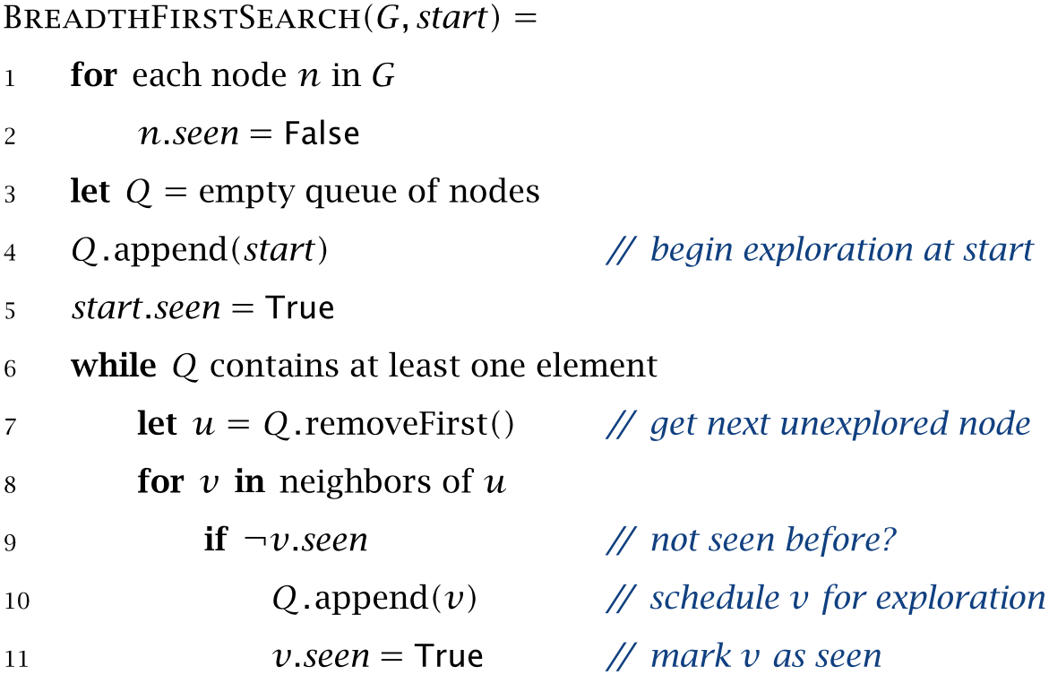
The algorithm then processes the starting node start by adding it to the queue and marking it as seen. Most of the work is done by the outer while loop, which continues as long as there are unexplored nodes in \(Q\). In each iteration, the node at the
front of the queue is removed and explored. The first iteration always explores start, since this is the only element in \(Q\); in subsequent iterations, the queue contains the neighbors of start, then the neighbors of the neighbors, and so on. A particular node \(u\) is explored by
inspecting its neighbors in the graph. Each neighbor \(v\) that hasn’t been encountered before is added to \(Q\) for later exploration and then marked as seen. The algorithm continues until \(Q\) is empty and all nodes in the graph that are reachable from start have been
visited.
The scan() method in Listing 7.5 illustrates one possible implementation of breadth-first search. The method traverses a Graph starting at node start until it finds a node that satisfies a certain condition. This condition is provided as an argument of type Predicate and can be specified by the caller of scan(); we will discuss predicates in more detail below. The code uses two main data structures. The first is unexplored, implemented using Java’s ArrayDeque class, which corresponds to the \(Q\) variable in Algorithm 7.1 and holds all nodes that still need to be explored in first-in first-out order. The second is the HashSet seen, which keeps track of all nodes that have been encountered by the algorithm so far; this set replaces the seen field used in Algorithm 7.1.
// Scan all nodes that are reachable from 'start'. Stop when
// 'condition' is satisfied.
default N scan(N start, Predicate<N> condition) {
    var seen = new HashSet<>(List.of(start));
    var unexplored = new ArrayDeque<>(List.of(start));
    while (!unexplored.isEmpty()) {
        N node = unexplored.removeFirst();
        if (condition.test(node))
            return node;
        for (N neighbor : neighbors(node)) {
            if (seen.add(neighbor))
                unexplored.addLast(neighbor);
        }
    }
    return null;
}
In each iteration of the main loop, scan() removes one node from the start of the queue. If it satisfies the search condition, the traversal is stopped immediately and node is returned as
the search result. Otherwise, all neighbors of node that haven’t been seen before are added to the unexplored queue. The return statement at the end of the function is only reached if none of the reachable nodes satisfy the search condition; in this case, the search
fails and scan() returns null.
The second argument to scan() is the search condition. The type Predicate is a so-called functional interface that describes functions that take a single argument of type N and return a boolean value. (See Appendix B.6 for an overview of functional interfaces and predefined function types such as Predicate.) The use of a predicate argument makes it possible to customize the
behavior of scan() from the outside. Effectively, the method implements a generalized version of breadth-first search that delegates part of the algorithm — the decisions when to stop the traversal
and what action to perform when a new node is visited — to the function condition.
If we call scan() with a predicate that always returns false, breadth-first search runs until all nodes that are reachable from the start have been visited. This is such a
common and useful operation that we provide it as a dedicated function visitNodes() in Listing 7.6. The second argument of
visitNodes() is a Consumer, a type of function that accepts a single value of type N but (unlike Predicate) doesn’t return a value.
The implementation of visitNodes() delegates the actual traversal to scan(), using a
predicate that always returns false to ensure that every reachable node is visited. In addition, the predicate hands over every node to consumer by calling its accept() method.
// Visit all nodes that are reachable from 'start'.
default void visitNodes(N start, Consumer<N> consumer) {
    scan(start, node -> {
        consumer.accept(node);
        return false;
    });
}
Let’s take a look at a few examples to see how scan() and visitNodes() can be used in
practice. We can find out whether the 43 node is reachable from the 00 node by calling scan() as follows:
if (new DieHardGraph().scan("00", "43"::equals) != null) {
    System.out.println("solution found");
}
The predicate passed to scan() is the expression "43"::equals, which is a reference to equals() method
of the string "43". With this predicate, scan() traverses the graph until it finds a node that matches "43".
We can print the nodes of the die-hard graph in the order they are encountered by breadth-first search by calling visitNodes() and
passing a reference to println() as the last argument:
new DieHardGraph().visitNodes("00", System.out::println);
// Output: 00 03 50 30 53 23 33 20 51 02 01 52 10 43 13 40
Alternatively, we can collect the reachable nodes in a list by specifying a function that appends each node to a given data structure:
var nodes = new ArrayList<>();
new DieHardGraph().visitNodes("00", nodes::add);
Every time visitNodes() reaches a new node, it calls the add() method associated with nodes.
The Anatomy of Graphs
There is a useful variation of breadth-first search that groups reachable nodes by their distance from the start. Instead of processing nodes and their neighbors one by one, this variation first determines all nodes at distance 1 from the start, then all nodes at
distance 2, then all nodes at distance 3, and so on. We refer to the set of all nodes at a fixed distance from a certain node as a layer and represent it using the GraphLayer type defined in Listing 7.7.
Listing 7.7ch7 / GraphLayer
// The set of nodes at a certain distance from 'start'.
public record GraphLayer<N>(
        N start,
        int distance,
        List<N> nodes) {
}
The scanLayers() method in Listing 7.8 traverses a graph layer by layer until a certain condition is met. The traversal starts at
the specified node start. The implementation of scanLayers() is similar to that of Graph.scan(), except that the outer loop now processes one layer at a time. In each iteration, we examine all neighbors of the current layer and add every newly discovered node to next; after processing the current layer, this becomes
the next layer of nodes. The loop stops when a layer that matches condition has been found or after the final layer has been processed. Notice that this version of breadth-first search doesn’t require the use of a queue to maintain
the list of unexplored nodes.
// Scan all layers reachable from 'start' and stop at the first one
// that satisfies 'condition'.
default GraphLayer<N> scanLayers(N start,
        Predicate<GraphLayer<N>> condition) {
    var seen = new HashSet<>(List.of(start));
    var next = new ArrayList<N>();
    next.add(start);
    for (int distance = 0; !next.isEmpty(); distance++) {
        var layer = new GraphLayer<>(start, distance, next);
        if (condition.test(layer))
            return layer;
        next = new ArrayList<>();
        for (var node : layer.nodes()) {
            for (N neighbor : neighbors(node)) {
                if (seen.add(neighbor))
                    next.add(neighbor);
            }
        }
    }
    return null;
}
We also define an an additional method visitLayers() that unconditionally visits every layer that is reachable from start (Listing 7.9).
// Visit all layers reachable from 'start'.
default void visitLayers(N start, Consumer<GraphLayer<N>> consumer) {
    scanLayers(start, layer -> {
        consumer.accept(layer);
        return false;
    });
}
Let’s use these two functions to explore the die-hard graph further. Maybe the simplest application of visitLayers() is to print all layers that are reachable from
node 00:
var graph = new DieHardGraph();
graph.visitLayers("00", System.out::println);
The output agrees with the table in Fig. 7.1: all 16 nodes can be reached in seven steps or less, and the first node in which one of the jugs contains four gallons is found in the layer at distance 6.
GraphLayer[distance=0, start=00, nodes=[00]]
GraphLayer[distance=1, start=00, nodes=[03, 50]]
GraphLayer[distance=2, start=00, nodes=[30, 53, 23]]
GraphLayer[distance=3, start=00, nodes=[33, 20]]
GraphLayer[distance=4, start=00, nodes=[51, 02]]
GraphLayer[distance=5, start=00, nodes=[01, 52]]
GraphLayer[distance=6, start=00, nodes=[10, 43]]
GraphLayer[distance=7, start=00, nodes=[13, 40]]
What happens if we start at another node, for example node 10?
graph.visitLayers("10", System.out::println);
In this case, we can still reach all 16 nodes, but now we need four steps at most, and the original problem of measuring four gallons becomes almost trivial, requiring only two steps:
GraphLayer[distance=0, start=10, nodes=[10]]
GraphLayer[distance=1, start=10, nodes=[00, 01, 13, 50]]
GraphLayer[distance=2, start=10, nodes=[03, 51, 40, 53, 23]]
GraphLayer[distance=3, start=10, nodes=[30, 33, 43, 20]]
GraphLayer[distance=4, start=10, nodes=[52, 02]]
For a given node \(n\), the maximum number of steps it takes to reach any other node of the graph is known as that node’s eccentricity \(\epsilon (n)\). (We just saw that the nodes 00 and 10 in the die-hard graph have the eccentricities 7 and 4, respectively.) In general, the eccentricity tells us how a node is
positioned relative to all other nodes in the graph. A small value of \(\epsilon (n)\) indicates that \(n\) close to every reachable node, whereas a large value means that \(n\) is far away from (at least) one node. The eccentricity therefore allows us to distinguish between the center of the graph
(small \(\epsilon \)) and its periphery (large \(\epsilon \)). Several important graph quantities are defined in terms of the eccentricity:
-
• The radius of a graph is the smallest eccentricity of any of its nodes.
-
• The center of a graph is the set of nodes whose eccentricity equals the graph’s radius.
-
• The diameter of a graph is the largest eccentricity of any of its nodes. This is the length of the “longest shortest path” between any pair of nodes.
A small radius indicates that all nodes are close to its center, and a small diameter indicates that all nodes close to each other.
To compute the eccentricity of a node \(n\), we can use breadth-first search to traverse the graph starting at \(n\) and continue until no new nodes are discovered; the eccentricity is the distance from \(n\) to the last node that
was found. Alternatively, we can traverse the layers of the graph to find the one that is farthest from \(n\). The farthestLayer() method defined in Listing 7.10 computes this farthest layer by iterating over all layers using Graph.visitLayers() and keeping only the last one. (The
farthest variable must be defined inside an anonymous object result to work around the unfortunate limitation that lambda expressions in Java cannot modify local variables defined in the surrounding scope; for
more details about this technique, see the discussion in Appendix B.6.)
Listing 7.10ch7 / GraphUtil
// Find the set of nodes with the maximum distance from 'node'.
public static <N> GraphLayer<N> farthestLayer(Graph<N> graph, N node) {
    var result = new Object() {
        GraphLayer<N> farthest;
    };
    graph.visitLayers(node, layer -> result.farthest = layer);
    return result.farthest;
}
Using farthestLayer(), we can now define functions that compute a node’s eccentricity as well as a graph’s radius and diameter (Listing 7.11). The implementation of eccentricity() simply determines the layer farthest from
n and returns its distance, and the functions radius() and diameter()
compute the radius and diameter by iterating over all nodes and returning the smallest or largest eccentricity encountered.
Listing 7.11ch7 / GraphUtil
// Compute the eccentricity of the node n.
public static <N> int eccentricity(Graph<N> graph, N n) {
    return farthestLayer(graph, n).distance();
}

// Compute the radius of 'graph'.
public static <N> int radius(Graph<N> graph) {
    int min = Integer.MAX_VALUE;
    for (N node : graph.nodes()) {
        min = Math.min(min, eccentricity(graph, node));
    }
    return min;
}

// Compute the diameter of 'graph'.
public static <N> int diameter(Graph<N> graph) {
    int max = 0;
    for (N node : graph.nodes()) {
        max = Math.max(max, eccentricity(graph, node));
    }
    return max;
}
In the case of the die-hard graph, the smallest eccentricity, and therefore the graph’s radius, is 4. There are four nodes with this eccentricity: 10, 13, 40, and 43. They form the center of the graph, and
from them every other node can be reached in at most four steps. The diameter of the die-hard graph is 7, which means that the hardest measuring problems require seven steps. There are eight such problems:
| . |
|---|
| 00 to 13 |
00 to 40 |
03 to 43 |
03 to 40 |
| 50 to 10 |
50 to 13 |
53 to 13 |
53 to 40 |
A slightly harder version of the die-hard problem is therefore: Given an empty 5 gallon jug and a full 3 gallon jug, find a way to measure exactly four gallons of water. This is the hardest measuring problem for these two jugs.
Exercises
Exercise 7.3.True or false: The farthestLayer() method defined in Listing 7.10 never returns null.
Exercise 7.4.Compute the eccentricities of all nodes in the die-hard graph (Fig. 7.2).