7 Traversing Graphs

\(\newcommand{\footnotename}{footnote}\) \(\def \LWRfootnote {1}\) \(\newcommand {\footnote }[2][\LWRfootnote ]{{}^{\mathrm {#1}}}\) \(\newcommand {\footnotemark }[1][\LWRfootnote ]{{}^{\mathrm {#1}}}\) \(\let \LWRorighspace \hspace \) \(\renewcommand {\hspace }{\ifstar \LWRorighspace \LWRorighspace }\) \(\newcommand {\TextOrMath }[2]{#2}\) \(\newcommand {\mathnormal }[1]{{#1}}\) \(\newcommand \ensuremath [1]{#1}\) \(\newcommand {\LWRframebox }[2][]{\fbox {#2}} \newcommand {\framebox }[1][]{\LWRframebox } \) \(\newcommand {\setlength }[2]{}\) \(\newcommand {\addtolength }[2]{}\) \(\newcommand {\setcounter }[2]{}\) \(\newcommand {\addtocounter }[2]{}\) \(\newcommand {\arabic }[1]{}\) \(\newcommand {\number }[1]{}\) \(\newcommand {\noalign }[1]{\text {#1}\notag \\}\) \(\newcommand {\cline }[1]{}\) \(\newcommand {\directlua }[1]{\text {(directlua)}}\) \(\newcommand {\luatexdirectlua }[1]{\text {(directlua)}}\) \(\newcommand {\protect }{}\) \(\def \LWRabsorbnumber #1 {}\) \(\def \LWRabsorbquotenumber "#1 {}\) \(\newcommand {\LWRabsorboption }[1][]{}\) \(\newcommand {\LWRabsorbtwooptions }[1][]{\LWRabsorboption }\) \(\def \mathchar {\ifnextchar "\LWRabsorbquotenumber \LWRabsorbnumber }\) \(\def \mathcode #1={\mathchar }\) \(\let \delcode \mathcode \) \(\let \delimiter \mathchar \) \(\def \oe {\unicode {x0153}}\) \(\def \OE {\unicode {x0152}}\) \(\def \ae {\unicode {x00E6}}\) \(\def \AE {\unicode {x00C6}}\) \(\def \aa {\unicode {x00E5}}\) \(\def \AA {\unicode {x00C5}}\) \(\def \o {\unicode {x00F8}}\) \(\def \O {\unicode {x00D8}}\) \(\def \l {\unicode {x0142}}\) \(\def \L {\unicode {x0141}}\) \(\def \ss {\unicode {x00DF}}\) \(\def \SS {\unicode {x1E9E}}\) \(\def \dag {\unicode {x2020}}\) \(\def \ddag {\unicode {x2021}}\) \(\def \P {\unicode {x00B6}}\) \(\def \copyright {\unicode {x00A9}}\) \(\def \pounds {\unicode {x00A3}}\) \(\let \LWRref \ref \) \(\renewcommand {\ref }{\ifstar \LWRref \LWRref }\) \( \newcommand {\multicolumn }[3]{#3}\) \(\require {textcomp}\) \(\newcommand {\intertext }[1]{\text {#1}\notag \\}\) \(\let \Hat \hat \) \(\let \Check \check \) \(\let \Tilde \tilde \) \(\let \Acute \acute \) \(\let \Grave \grave \) \(\let \Dot \dot \) \(\let \Ddot \ddot \) \(\let \Breve \breve \) \(\let \Bar \bar \) \(\let \Vec \vec \) \(\renewcommand {\vec }{\boldsymbol }\) \(\newcommand {\Edge }{\ensuremath {\,\textemdash \,}}\) \(\newcommand \Const [1]{\text {\textsf {#1}}}\) \(\DeclareMathOperator {\lerp }{lerp}\) \(\DeclareMathOperator {\bitlen }{bitlen}\) \(\DeclareMathOperator {\sign }{sign}\) \(\newcommand {\I }{\mathrm {i}}\) \(\newcommand \AND {\mathbin {\&}}\) \(\newcommand \OR {\mathbin {|}}\) \(\newcommand \XOR {\mathbin {{}^{\wedge }}}\) \(\newcommand \shl {\ll }\) \(\newcommand \shr {\ggg }\) \(\newcommand \asr {\gg }\) \(\newcommand \NOT {\ensuremath {\mathord {\sim }}}\) \(\newcommand {\isep }{\mathrel {{.}\,{.}}}\) \(\newcommand {\Id }[1]{\mathit {#1}}\) \(\newcommand {\const }[1]{\mathsf {#1}}\) \(\newcommand {\algorithmname }[1]{\text {\textsc {#1}}}\) \(\newcommand {\bits }[1]{\text {#1}}\) \(\newcommand {\hexa }[1]{\mathtt {0x#1}}\) \(\newcommand {\num }[1]{#1}\) \(\newcommand {\qed }{\quad \square }\) \(\newcommand {\idiv }[2]{\lfloor #1/#2\rfloor }\) \(\newcommand \attribdot {\ensuremath {\mkern 1.5mu.\mkern 1.5mu}}\) \(\newcommand \attribxr [2]{#1\attribdot \text {#2}}\) \(\newcommand \attribir [2]{\Id {#1}\attribdot \text {#2}}\) \(\newcommand \attribii [2]{\Id {#1}\attribdot \Id {#2}}\) \(\newcommand \textsc [1]{#1}\) \(\require {colortbl}\) \(\let \LWRorigcolumncolor \columncolor \) \(\renewcommand {\columncolor }[2][named]{\LWRorigcolumncolor [#1]{#2}\LWRabsorbtwooptions }\) \(\let \LWRorigrowcolor \rowcolor \) \(\renewcommand {\rowcolor }[2][named]{\LWRorigrowcolor [#1]{#2}\LWRabsorbtwooptions }\) \(\let \LWRorigcellcolor \cellcolor \) \(\renewcommand {\cellcolor }[2][named]{\LWRorigcellcolor [#1]{#2}\LWRabsorbtwooptions }\) \(\newcommand {\tcbset }[1]{}\) \(\newcommand {\tcbsetforeverylayer }[1]{}\) \(\newcommand {\tcbox }[2][]{\boxed {\text {#2}}}\) \(\newcommand {\tcboxfit }[2][]{\boxed {#2}}\) \(\newcommand {\tcblower }{}\) \(\newcommand {\tcbline }{}\) \(\newcommand {\tcbtitle }{}\) \(\newcommand {\tcbsubtitle [2][]{\mathrm {#2}}}\) \(\newcommand {\tcboxmath }[2][]{\boxed {#2}}\) \(\newcommand {\tcbhighmath }[2][]{\boxed {#2}}\) \(\newcommand {\toprule }[1][]{\hline }\) \(\let \midrule \toprule \) \(\let \bottomrule \toprule \) \(\def \LWRbooktabscmidruleparen (#1)#2{}\) \(\newcommand {\LWRbooktabscmidrulenoparen }[1]{}\) \(\newcommand {\cmidrule }[1][]{\ifnextchar (\LWRbooktabscmidruleparen \LWRbooktabscmidrulenoparen }\) \(\newcommand {\morecmidrules }{}\) \(\newcommand {\specialrule }[3]{\hline }\) \(\newcommand {\addlinespace }[1][]{}\) \(\newcommand {\LWRsubmultirow }[2][]{#2}\) \(\newcommand {\LWRmultirow }[2][]{\LWRsubmultirow }\) \(\newcommand {\multirow }[2][]{\LWRmultirow }\) \(\newcommand {\mrowcell }{}\) \(\newcommand {\mcolrowcell }{}\) \(\newcommand {\STneed }[1]{}\) \(\newcommand {\LWRldelimtwo }[1][]{\text {#1}~\LWRbigdelim }\) \(\newcommand {\LWRldelimone }[2][]{\LWRldelimtwo }\) \(\def \ldelim #1#2{\def \LWRbigdelim {#1}\LWRldelimone }\) \(\newcommand {\LWRrdelimtwo }[1][]{\LWRbigdelim ~\text {#1}}\) \(\newcommand {\LWRrdelimone }[2][]{\LWRrdelimtwo }\) \(\def \rdelim #1#2{\def \LWRbigdelim {#1}\LWRrdelimone }\) \(\let \symnormal \mathit \) \(\let \symliteral \mathrm \) \(\let \symbb \mathbb \) \(\let \symbbit \mathbb \) \(\let \symcal \mathcal \) \(\let \symscr \mathscr \) \(\let \symfrak \mathfrak \) \(\let \symsfup \mathsf \) \(\let \symsfit \mathit \) \(\let \symbfsf \mathbf \) \(\let \symbfup \mathbf \) \(\newcommand {\symbfit }[1]{\boldsymbol {#1}}\) \(\let \symbfcal \mathcal \) \(\let \symbfscr \mathscr \) \(\let \symbffrak \mathfrak \) \(\let \symbfsfup \mathbf \) \(\newcommand {\symbfsfit }[1]{\boldsymbol {#1}}\) \(\let \symup \mathrm \) \(\let \symbf \mathbf \) \(\let \symit \mathit \) \(\let \symsf \symsfit \) \(\let \symtt \mathtt \) \(\let \symbffrac \mathbffrac \) \(\newcommand {\mathfence }[1]{\mathord {#1}}\) \(\newcommand {\mathover }[1]{#1}\) \(\newcommand {\mathunder }[1]{#1}\) \(\newcommand {\mathaccent }[1]{#1}\) \(\newcommand {\mathbotaccent }[1]{#1}\) \(\newcommand {\mathalpha }[1]{\mathord {#1}}\) \(\def\Alpha{\unicode{x1D6E2}}\) \(\def\Beta{\unicode{x1D6E3}}\) \(\def\Gamma{\unicode{x1D6E4}}\) \(\def\Digamma{\mathit{\unicode{x03DC}}}\) \(\def\Delta{\unicode{x1D6E5}}\) \(\def\Epsilon{\unicode{x1D6E6}}\) \(\def\Zeta{\unicode{x1D6E7}}\) \(\def\Eta{\unicode{x1D6E8}}\) \(\def\Theta{\unicode{x1D6E9}}\) \(\def\Vartheta{\unicode{x1D6F3}}\) \(\def\Iota{\unicode{x1D6EA}}\) \(\def\Kappa{\unicode{x1D6EB}}\) \(\def\Lambda{\unicode{x1D6EC}}\) \(\def\Mu{\unicode{x1D6ED}}\) \(\def\Nu{\unicode{x1D6EE}}\) \(\def\Xi{\unicode{x1D6EF}}\) \(\def\Omicron{\unicode{x1D6F0}}\) \(\def\Pi{\unicode{x1D6F1}}\) \(\def\Rho{\unicode{x1D6F2}}\) \(\def\Sigma{\unicode{x1D6F4}}\) \(\def\Tau{\unicode{x1D6F5}}\) \(\def\Upsilon{\unicode{x1D6F6}}\) \(\def\Phi{\unicode{x1D6F7}}\) \(\def\Chi{\unicode{x1D6F8}}\) \(\def\Psi{\unicode{x1D6F9}}\) \(\def\Omega{\unicode{x1D6FA}}\) \(\def\alpha{\unicode{x1D6FC}}\) \(\def\beta{\unicode{x1D6FD}}\) \(\def\varbeta{\unicode{x03D0}}\) \(\def\gamma{\unicode{x1D6FE}}\) \(\def\digamma{\mathit{\unicode{x03DD}}}\) \(\def\delta{\unicode{x1D6FF}}\) \(\def\epsilon{\unicode{x1D716}}\) \(\def\varepsilon{\unicode{x1D700}}\) \(\def\zeta{\unicode{x1D701}}\) \(\def\eta{\unicode{x1D702}}\) \(\def\theta{\unicode{x1D703}}\) \(\def\vartheta{\unicode{x1D717}}\) \(\def\iota{\unicode{x1D704}}\) \(\def\kappa{\unicode{x1D705}}\) \(\def\varkappa{\unicode{x1D718}}\) \(\def\lambda{\unicode{x1D706}}\) \(\def\mu{\unicode{x1D707}}\) \(\def\nu{\unicode{x1D708}}\) \(\def\xi{\unicode{x1D709}}\) \(\def\omicron{\unicode{x1D70A}}\) \(\def\pi{\unicode{x1D70B}}\) \(\def\varpi{\unicode{x1D71B}}\) \(\def\rho{\unicode{x1D70C}}\) \(\def\varrho{\unicode{x1D71A}}\) \(\def\sigma{\unicode{x1D70E}}\) \(\def\varsigma{\unicode{x1D70D}}\) \(\def\tau{\unicode{x1D70F}}\) \(\def\upsilon{\unicode{x1D710}}\) \(\def\phi{\unicode{x1D719}}\) \(\def\varphi{\unicode{x1D711}}\) \(\def\chi{\unicode{x1D712}}\) \(\def\psi{\unicode{x1D713}}\) \(\def\omega{\unicode{x1D714}}\) \(\def\upAlpha{\unicode{x0391}}\) \(\def\upBeta{\unicode{x0392}}\) \(\def\upGamma{\unicode{x0393}}\) \(\def\upDigamma{\unicode{x03DC}}\) \(\def\upDelta{\unicode{x0394}}\) \(\def\upEpsilon{\unicode{x0395}}\) \(\def\upZeta{\unicode{x0396}}\) \(\def\upEta{\unicode{x0397}}\) \(\def\upTheta{\unicode{x0398}}\) \(\def\upVartheta{\unicode{x03F4}}\) \(\def\upIota{\unicode{x0399}}\) \(\def\upKappa{\unicode{x039A}}\) \(\def\upLambda{\unicode{x039B}}\) \(\def\upMu{\unicode{x039C}}\) \(\def\upNu{\unicode{x039D}}\) \(\def\upXi{\unicode{x039E}}\) \(\def\upOmicron{\unicode{x039F}}\) \(\def\upPi{\unicode{x03A0}}\) \(\def\upVarpi{\unicode{x03D6}}\) \(\def\upRho{\unicode{x03A1}}\) \(\def\upSigma{\unicode{x03A3}}\) \(\def\upTau{\unicode{x03A4}}\) \(\def\upUpsilon{\unicode{x03A5}}\) \(\def\upPhi{\unicode{x03A6}}\) \(\def\upChi{\unicode{x03A7}}\) \(\def\upPsi{\unicode{x03A8}}\) \(\def\upOmega{\unicode{x03A9}}\) \(\def\itAlpha{\unicode{x1D6E2}}\) \(\def\itBeta{\unicode{x1D6E3}}\) \(\def\itGamma{\unicode{x1D6E4}}\) \(\def\itDigamma{\mathit{\unicode{x03DC}}}\) \(\def\itDelta{\unicode{x1D6E5}}\) \(\def\itEpsilon{\unicode{x1D6E6}}\) \(\def\itZeta{\unicode{x1D6E7}}\) \(\def\itEta{\unicode{x1D6E8}}\) \(\def\itTheta{\unicode{x1D6E9}}\) \(\def\itVartheta{\unicode{x1D6F3}}\) \(\def\itIota{\unicode{x1D6EA}}\) \(\def\itKappa{\unicode{x1D6EB}}\) \(\def\itLambda{\unicode{x1D6EC}}\) \(\def\itMu{\unicode{x1D6ED}}\) \(\def\itNu{\unicode{x1D6EE}}\) \(\def\itXi{\unicode{x1D6EF}}\) \(\def\itOmicron{\unicode{x1D6F0}}\) \(\def\itPi{\unicode{x1D6F1}}\) \(\def\itRho{\unicode{x1D6F2}}\) \(\def\itSigma{\unicode{x1D6F4}}\) \(\def\itTau{\unicode{x1D6F5}}\) \(\def\itUpsilon{\unicode{x1D6F6}}\) \(\def\itPhi{\unicode{x1D6F7}}\) \(\def\itChi{\unicode{x1D6F8}}\) \(\def\itPsi{\unicode{x1D6F9}}\) \(\def\itOmega{\unicode{x1D6FA}}\) \(\def\upalpha{\unicode{x03B1}}\) \(\def\upbeta{\unicode{x03B2}}\) \(\def\upvarbeta{\unicode{x03D0}}\) \(\def\upgamma{\unicode{x03B3}}\) \(\def\updigamma{\unicode{x03DD}}\) \(\def\updelta{\unicode{x03B4}}\) \(\def\upepsilon{\unicode{x03F5}}\) \(\def\upvarepsilon{\unicode{x03B5}}\) \(\def\upzeta{\unicode{x03B6}}\) \(\def\upeta{\unicode{x03B7}}\) \(\def\uptheta{\unicode{x03B8}}\) \(\def\upvartheta{\unicode{x03D1}}\) \(\def\upiota{\unicode{x03B9}}\) \(\def\upkappa{\unicode{x03BA}}\) \(\def\upvarkappa{\unicode{x03F0}}\) \(\def\uplambda{\unicode{x03BB}}\) \(\def\upmu{\unicode{x03BC}}\) \(\def\upnu{\unicode{x03BD}}\) \(\def\upxi{\unicode{x03BE}}\) \(\def\upomicron{\unicode{x03BF}}\) \(\def\uppi{\unicode{x03C0}}\) \(\def\upvarpi{\unicode{x03D6}}\) \(\def\uprho{\unicode{x03C1}}\) \(\def\upvarrho{\unicode{x03F1}}\) \(\def\upsigma{\unicode{x03C3}}\) \(\def\upvarsigma{\unicode{x03C2}}\) \(\def\uptau{\unicode{x03C4}}\) \(\def\upupsilon{\unicode{x03C5}}\) \(\def\upphi{\unicode{x03D5}}\) \(\def\upvarphi{\unicode{x03C6}}\) \(\def\upchi{\unicode{x03C7}}\) \(\def\uppsi{\unicode{x03C8}}\) \(\def\upomega{\unicode{x03C9}}\) \(\def\italpha{\unicode{x1D6FC}}\) \(\def\itbeta{\unicode{x1D6FD}}\) \(\def\itvarbeta{\unicode{x03D0}}\) \(\def\itgamma{\unicode{x1D6FE}}\) \(\def\itdigamma{\mathit{\unicode{x03DD}}}\) \(\def\itdelta{\unicode{x1D6FF}}\) \(\def\itepsilon{\unicode{x1D716}}\) \(\def\itvarepsilon{\unicode{x1D700}}\) \(\def\itzeta{\unicode{x1D701}}\) \(\def\iteta{\unicode{x1D702}}\) \(\def\ittheta{\unicode{x1D703}}\) \(\def\itvartheta{\unicode{x1D717}}\) \(\def\itiota{\unicode{x1D704}}\) \(\def\itkappa{\unicode{x1D705}}\) \(\def\itvarkappa{\unicode{x1D718}}\) \(\def\itlambda{\unicode{x1D706}}\) \(\def\itmu{\unicode{x1D707}}\) \(\def\itnu{\unicode{x1D708}}\) \(\def\itxi{\unicode{x1D709}}\) \(\def\itomicron{\unicode{x1D70A}}\) \(\def\itpi{\unicode{x1D70B}}\) \(\def\itvarpi{\unicode{x1D71B}}\) \(\def\itrho{\unicode{x1D70C}}\) \(\def\itvarrho{\unicode{x1D71A}}\) \(\def\itsigma{\unicode{x1D70E}}\) \(\def\itvarsigma{\unicode{x1D70D}}\) \(\def\ittau{\unicode{x1D70F}}\) \(\def\itupsilon{\unicode{x1D710}}\) \(\def\itphi{\unicode{x1D719}}\) \(\def\itvarphi{\unicode{x1D711}}\) \(\def\itchi{\unicode{x1D712}}\) \(\def\itpsi{\unicode{x1D713}}\) \(\def\itomega{\unicode{x1D714}}\) \(\let \lparen (\) \(\let \rparen )\) \(\newcommand {\cuberoot }[1]{\,{}^3\!\!\sqrt {#1}}\,\) \(\newcommand {\fourthroot }[1]{\,{}^4\!\!\sqrt {#1}}\,\) \(\newcommand {\longdivision }[1]{\mathord {\unicode {x027CC}#1}}\) \(\newcommand {\mathcomma }{,}\) \(\newcommand {\mathcolon }{:}\) \(\newcommand {\mathsemicolon }{;}\) \(\newcommand {\overbracket }[1]{\mathinner {\overline {\ulcorner {#1}\urcorner }}}\) \(\newcommand {\underbracket }[1]{\mathinner {\underline {\llcorner {#1}\lrcorner }}}\) \(\newcommand {\overbar }[1]{\mathord {#1\unicode {x00305}}}\) \(\newcommand {\ovhook }[1]{\mathord {#1\unicode {x00309}}}\) \(\newcommand {\ocirc }[1]{\mathord {#1\unicode {x0030A}}}\) \(\newcommand {\candra }[1]{\mathord {#1\unicode {x00310}}}\) \(\newcommand {\oturnedcomma }[1]{\mathord {#1\unicode {x00312}}}\) \(\newcommand {\ocommatopright }[1]{\mathord {#1\unicode {x00315}}}\) \(\newcommand {\droang }[1]{\mathord {#1\unicode {x0031A}}}\) \(\newcommand {\leftharpoonaccent }[1]{\mathord {#1\unicode {x020D0}}}\) \(\newcommand {\rightharpoonaccent }[1]{\mathord {#1\unicode {x020D1}}}\) \(\newcommand {\vertoverlay }[1]{\mathord {#1\unicode {x020D2}}}\) \(\newcommand {\leftarrowaccent }[1]{\mathord {#1\unicode {x020D0}}}\) \(\newcommand {\annuity }[1]{\mathord {#1\unicode {x020E7}}}\) \(\newcommand {\widebridgeabove }[1]{\mathord {#1\unicode {x020E9}}}\) \(\newcommand {\asteraccent }[1]{\mathord {#1\unicode {x020F0}}}\) \(\newcommand {\threeunderdot }[1]{\mathord {#1\unicode {x020E8}}}\) \(\newcommand {\Bbbsum }{\mathop {\unicode {x2140}}\limits }\) \(\newcommand {\oiint }{\mathop {\unicode {x222F}}\limits }\) \(\newcommand {\oiiint }{\mathop {\unicode {x2230}}\limits }\) \(\newcommand {\intclockwise }{\mathop {\unicode {x2231}}\limits }\) \(\newcommand {\ointclockwise }{\mathop {\unicode {x2232}}\limits }\) \(\newcommand {\ointctrclockwise }{\mathop {\unicode {x2233}}\limits }\) \(\newcommand {\varointclockwise }{\mathop {\unicode {x2232}}\limits }\) \(\newcommand {\leftouterjoin }{\mathop {\unicode {x27D5}}\limits }\) \(\newcommand {\rightouterjoin }{\mathop {\unicode {x27D6}}\limits }\) \(\newcommand {\fullouterjoin }{\mathop {\unicode {x27D7}}\limits }\) \(\newcommand {\bigbot }{\mathop {\unicode {x27D8}}\limits }\) \(\newcommand {\bigtop }{\mathop {\unicode {x27D9}}\limits }\) \(\newcommand {\xsol }{\mathop {\unicode {x29F8}}\limits }\) \(\newcommand {\xbsol }{\mathop {\unicode {x29F9}}\limits }\) \(\newcommand {\bigcupdot }{\mathop {\unicode {x2A03}}\limits }\) \(\newcommand {\bigsqcap }{\mathop {\unicode {x2A05}}\limits }\) \(\newcommand {\conjquant }{\mathop {\unicode {x2A07}}\limits }\) \(\newcommand {\disjquant }{\mathop {\unicode {x2A08}}\limits }\) \(\newcommand {\bigtimes }{\mathop {\unicode {x2A09}}\limits }\) \(\newcommand {\modtwosum }{\mathop {\unicode {x2A0A}}\limits }\) \(\newcommand {\sumint }{\mathop {\unicode {x2A0B}}\limits }\) \(\newcommand {\intbar }{\mathop {\unicode {x2A0D}}\limits }\) \(\newcommand {\intBar }{\mathop {\unicode {x2A0E}}\limits }\) \(\newcommand {\fint }{\mathop {\unicode {x2A0F}}\limits }\) \(\newcommand {\cirfnint }{\mathop {\unicode {x2A10}}\limits }\) \(\newcommand {\awint }{\mathop {\unicode {x2A11}}\limits }\) \(\newcommand {\rppolint }{\mathop {\unicode {x2A12}}\limits }\) \(\newcommand {\scpolint }{\mathop {\unicode {x2A13}}\limits }\) \(\newcommand {\npolint }{\mathop {\unicode {x2A14}}\limits }\) \(\newcommand {\pointint }{\mathop {\unicode {x2A15}}\limits }\) \(\newcommand {\sqint }{\mathop {\unicode {x2A16}}\limits }\) \(\newcommand {\intlarhk }{\mathop {\unicode {x2A17}}\limits }\) \(\newcommand {\intx }{\mathop {\unicode {x2A18}}\limits }\) \(\newcommand {\intcap }{\mathop {\unicode {x2A19}}\limits }\) \(\newcommand {\intcup }{\mathop {\unicode {x2A1A}}\limits }\) \(\newcommand {\upint }{\mathop {\unicode {x2A1B}}\limits }\) \(\newcommand {\lowint }{\mathop {\unicode {x2A1C}}\limits }\) \(\newcommand {\bigtriangleleft }{\mathop {\unicode {x2A1E}}\limits }\) \(\newcommand {\zcmp }{\mathop {\unicode {x2A1F}}\limits }\) \(\newcommand {\zpipe }{\mathop {\unicode {x2A20}}\limits }\) \(\newcommand {\zproject }{\mathop {\unicode {x2A21}}\limits }\) \(\newcommand {\biginterleave }{\mathop {\unicode {x2AFC}}\limits }\) \(\newcommand {\bigtalloblong }{\mathop {\unicode {x2AFF}}\limits }\) \(\newcommand {\arabicmaj }{\mathop {\unicode {x1EEF0}}\limits }\) \(\newcommand {\arabichad }{\mathop {\unicode {x1EEF1}}\limits }\)

7.4 Problems

River-Crossing Problems

Exercise 7.6.One of the oldest known mathematical puzzles is the wolf-goat-cabbage problem. At the break of dawn, a farmer sets out for the market in a nearby village. She is accompanied by a small goat and a domesticated wolf, and she is carrying a large cabbage she hopes to sell at the market. To reach the village, the unconventional party has to cross a river using a small boat that is just large enough to carry the farmer and either the wolf, the goat, or the cabbage. For obvious reasons, the farmer cannot leave the goat alone with the cabbage or the wolf alone with the goat.

  • a) Is there still a way for the whole party to cross the river unharmed?

Although it’s fairly easy to solve the wolf-goat-cabbage problem by hand, it’s even easier when modeling it using graphs. The idea, again, is to enumerate the possible states of the problem and study how they are connected by valid moves.

  • b) How many different states are there? Propose a way to label them.

  • c) Construct the graph that underlies the wolf-goat-cabbage problem and explain why it is symmetric. How many different solutions are there?

  • d) Implement the resulting graph using the Graph interface.

Exercise 7.7.Here is another river-crossing puzzle that is similar to the wolf-goat-cabbage problem but uses different constraints on who may use the boat at a given time. It is called the jealous couples problem.

Two married couples need to cross a river. There is a small rowing boat that holds a maximum of two people. To group agrees on the following rule so that no one is getting jealous: No wife should ever be left in the presence of another man unless her husband is present as well.

  • a) Is it possible for both couples to get across the river without anyone getting jealous? How many trips are necessary?

The puzzle can be extended to an arbitrary number of couples. With three jealous couples, it is still possible to cross the river, but when there are four or more couples, the problem has no solution. A popular variation of the puzzle is therefore to add an island in the middle of the stream that can be used to drop off passengers, should the need arise.

  • b) Write a program that solves the jealous couples problem with an island. Your program should be able to handle at least ten couples.

  • c) Use your program to study the \(n\)-couple problem with an island for \(2\le n\le 10\). For which values of \(n\) is there a solution, and how many trips are required in each case?

Measuring with Three Jugs

Exercise 7.8.Consider the following variation of the die-hard problem. There are now three jugs: two empty jugs that can hold three and five gallons, respectively, and an additional jug that is filled with eight gallons of water. (This third jug replaces the fountain in the original description of the problem.) The goal is to evenly divide the contents of the eight-gallon jug.

  • a) What’s the relationship between this problem and the original die-hard problem?

  • b) Assume you start with only six gallons of water in the additional jug. Sketch the graph that corresponds to this problem. How does it differ from the die-hard graph in Fig. 7.2? Is it still possible to measure four gallons in this case? Is it possible to divide the six gallons evenly? If yes, what is the most efficient way of doing so?

  • c) Write a program that computes the graphs that model the three-jug problem. The structure of each graph is determined by four numbers: the capacities of the three jugs and the total amount of water distributed among the jugs. Explain how to compute the set of all nodes and the neighbors of each node.

  • d) Consider the three-jug problem with 6 units of water discussed in part (b). What is the diameter of the corresponding graph? What are the most difficult water-measuring problems of this puzzle?

Hanoi Graphs

Exercise 7.9.In Exercise 3.8 we discussed the Towers of Hanoi and how to solve this puzzle using recursion. In this exercise, we translate the puzzle into a graph problem and study the resulting Hanoi graph.

The Hanoi graph \(\text {Hanoi}(n)\) is defined as the graph that corresponds to the Towers of Hanoi puzzle with \(n\) disks. There is one node for each valid configuration of the \(n\) disks, and two nodes are connected by an edge if there is a legal move of a single disk that connects the corresponding disk configurations. The edges are undirected because all moves are reversible.

As we discussed in Exercise 3.8, every configuration of \(n\) disks (and therefore every node) can be described by a sequence of \(n\) letters that specifies the order in which disks are placed on the pegs A, B, and C. The node ABB corresponds to the configuration in which the largest disk is placed on peg A and the next two disks on peg B; peg C remains empty.

The first two Hanoi graphs are shown in Fig. 7.4. For \(n=1\) the graph consists of three nodes A, B, and C, and since the disk can be moved freely, there is an edge between each pair of nodes. For \(n=2\) there are nine nodes AA, AB, AC, BA, BB, BC, CA, CB, CC and a total of 12 edges between them. Nine of these 12 edges, including BA — BB, BB — BC, BC — BA, correspond to moving the small disk; the nodes that are connected by these edges differ in their last letter only. The remaining three edges AC — BC, AB — CB, and BA — CA correspond to moving the large disk, which is only possible if the small disk is out of the way.

Figure 7.4 The first two Hanoi graphs. There is one node for every configuration of disks, and an edge for every pair of configurations that are related by moving a single disk.

In general, every Hanoi graph \(\text {Hanoi}(n)\) consists of three smaller Hanoi graphs \(\text {Hanoi}(n-1)\) in which the largest disk remains fixed and the remaining \(n-1\) disks can move around freely. These three subgraphs are then joined by three edges that corresponds to moving the largest disk to a different peg. It’s easy to see that moving from one corner of the Hanoi graph to another corresponds to transferring every disk from one peg to another.

  • a) Sketch \(\text {Hanoi}(3)\). How many nodes and edges does the graph \(\text {Hanoi}(n)\) have?

  • b) Write a program that computes the Hanoi graph of order \(n\).

Using Hanoi graphs, we can solve the Towers of Hanoi by using breadth-first search to find a path from a starting node such as AAA to a target node such as CCC.

  • c) How efficient is breadth-first search compared to a tailor-made algorithm for solving the Towers of Hanoi such as the one we discussed in Exercise 3.8? Hint: Consider the number of nodes that are visited by both algorithms.

A path visits every node of a graph is called a Hamiltonian path, and a path that visits every node and returns to the start is a Hamiltonian cycle. It’s obvious that \(\text {A}\to {}\text {B}\to {}\text {C}\to {}\text {A}\) is a Hamiltonian cycle of \(\text {Hanoi}(1)\): the path is cyclic and contains all three nodes.

  • d) Find Hamiltonian cycles in \(\text {Hanoi}(2)\) and \(\text {Hanoi}(3)\).

  • e) Use induction to show that for every Hanoi graph it is possible to construct a Hamiltonian path between any two of its corners. Does every Hanoi graph also contain a Hamiltonian cycle?

Flood Fill

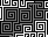
Exercise 7.10.Most paint programs come with a tool for filling regions of an image: The user clicks on a pixel inside the image, and the entire region connected to that pixel is filled with a new color. This operation is usually referred to as flood fill because its effect is reminiscent of color streaming out of the selected pixel and into neighboring pixels in all four directions until it is stopped by a different color. The two images in Fig. 7.5 illustrate how flood fill works. When the user clicks on one of the white pixels in the center of the maze, all white pixels that are directly or indirectly connected to it are set to a new color. Two pixels are only considered connected if they are horizontally or vertically adjacent, but not if they are diagonally adjacent.

(image)   (image)

Figure 7.5 Flood fill finds and colors a contiguous region of pixels in a raster image. One such region is shown in gray.

The simplest algorithm for flood fill uses an approach similar to breadth-first search. The main data structure is a queue of pixels in the image that is initialized to the pixel clicked by the user. Each step of the algorithm removes one pixel from this queue and inspect its four direct neighbors: Every neighbor that has the same color as the current pixel (or, by extension, the starting pixel), it added to the back of the queue. We then set the current pixel to its new color and repeat the process until the queue is empty. The pixels in the queue are always on the boundary of the flooded area, which expands outwards from the initial pixel.

  • a) Implement the flood fill algorithm. What happens in your implementation if the starting pixel already matches the new color?

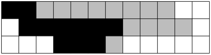
This simple flood fill algorithm is fairly slow and consumes a lot of memory when working with large images because it has to process every pixel individually. More efficient algorithms can be obtained by processing multiple pixels at once. One such approach is based on the idea of a span, a contiguous row of pixels with the same color. Two spans are considered adjacent if any of their pixels are adjacent and have the same color.

  • b) Consider the three rows of pixels shown in the following image:

    (-tikz- diagram)

    How many spans are there and which spans are adjacent to each other?

  • c) Modify your implementation of flood fill to work with spans instead of individual pixels. Each entry in the queue represents a single span, and each step of the algorithm fills an entire span and adds neighboring spans to the back of the queue.