\(\newcommand{\footnotename}{footnote}\) \(\def \LWRfootnote {1}\) \(\newcommand {\footnote }[2][\LWRfootnote ]{{}^{\mathrm {#1}}}\) \(\newcommand {\footnotemark }[1][\LWRfootnote ]{{}^{\mathrm {#1}}}\) \(\let \LWRorighspace \hspace \) \(\renewcommand {\hspace }{\ifstar \LWRorighspace \LWRorighspace }\) \(\newcommand {\TextOrMath }[2]{#2}\) \(\newcommand {\mathnormal }[1]{{#1}}\) \(\newcommand \ensuremath [1]{#1}\) \(\newcommand {\LWRframebox }[2][]{\fbox {#2}} \newcommand {\framebox }[1][]{\LWRframebox } \) \(\newcommand {\setlength }[2]{}\) \(\newcommand {\addtolength }[2]{}\) \(\newcommand {\setcounter }[2]{}\) \(\newcommand {\addtocounter }[2]{}\) \(\newcommand {\arabic }[1]{}\) \(\newcommand {\number }[1]{}\) \(\newcommand {\noalign }[1]{\text {#1}\notag \\}\) \(\newcommand {\cline }[1]{}\) \(\newcommand {\directlua }[1]{\text {(directlua)}}\) \(\newcommand {\luatexdirectlua }[1]{\text {(directlua)}}\) \(\newcommand {\protect }{}\) \(\def \LWRabsorbnumber #1 {}\) \(\def \LWRabsorbquotenumber "#1 {}\) \(\newcommand {\LWRabsorboption }[1][]{}\) \(\newcommand {\LWRabsorbtwooptions }[1][]{\LWRabsorboption }\) \(\def \mathchar {\ifnextchar "\LWRabsorbquotenumber \LWRabsorbnumber }\) \(\def \mathcode #1={\mathchar }\) \(\let \delcode \mathcode \) \(\let \delimiter \mathchar \) \(\def \oe {\unicode {x0153}}\) \(\def \OE {\unicode {x0152}}\) \(\def \ae {\unicode {x00E6}}\) \(\def \AE {\unicode {x00C6}}\) \(\def \aa {\unicode {x00E5}}\) \(\def \AA {\unicode {x00C5}}\) \(\def \o {\unicode {x00F8}}\) \(\def \O {\unicode {x00D8}}\) \(\def \l {\unicode {x0142}}\) \(\def \L {\unicode {x0141}}\) \(\def \ss {\unicode {x00DF}}\) \(\def \SS {\unicode {x1E9E}}\) \(\def \dag {\unicode {x2020}}\) \(\def \ddag {\unicode {x2021}}\) \(\def \P {\unicode {x00B6}}\) \(\def \copyright {\unicode {x00A9}}\) \(\def \pounds {\unicode {x00A3}}\) \(\let \LWRref \ref \) \(\renewcommand {\ref }{\ifstar \LWRref \LWRref }\) \( \newcommand {\multicolumn }[3]{#3}\) \(\require {textcomp}\) \(\newcommand {\intertext }[1]{\text {#1}\notag \\}\) \(\let \Hat \hat \) \(\let \Check \check \) \(\let \Tilde \tilde \) \(\let \Acute \acute \) \(\let \Grave \grave \) \(\let \Dot \dot \) \(\let \Ddot \ddot \) \(\let \Breve \breve \) \(\let \Bar \bar \) \(\let \Vec \vec \) \(\renewcommand {\vec }{\boldsymbol }\) \(\newcommand {\Edge }{\ensuremath {\,\textemdash \,}}\) \(\newcommand \Const [1]{\text {\textsf {#1}}}\) \(\DeclareMathOperator {\lerp }{lerp}\) \(\DeclareMathOperator {\bitlen }{bitlen}\) \(\DeclareMathOperator {\sign }{sign}\) \(\newcommand {\I }{\mathrm {i}}\) \(\newcommand \AND {\mathbin {\&}}\) \(\newcommand \OR {\mathbin {|}}\) \(\newcommand \XOR {\mathbin {{}^{\wedge }}}\) \(\newcommand \shl {\ll }\) \(\newcommand \shr {\ggg }\) \(\newcommand \asr {\gg }\) \(\newcommand \NOT {\ensuremath {\mathord {\sim }}}\) \(\newcommand {\isep }{\mathrel {{.}\,{.}}}\) \(\newcommand {\Id }[1]{\mathit {#1}}\) \(\newcommand {\const }[1]{\mathsf {#1}}\) \(\newcommand {\algorithmname }[1]{\text {\textsc {#1}}}\) \(\newcommand {\bits }[1]{\text {#1}}\) \(\newcommand {\hexa }[1]{\mathtt {0x#1}}\) \(\newcommand {\num }[1]{#1}\) \(\newcommand {\qed }{\quad \square }\) \(\newcommand {\idiv }[2]{\lfloor #1/#2\rfloor }\) \(\newcommand \attribdot {\ensuremath {\mkern 1.5mu.\mkern 1.5mu}}\) \(\newcommand \attribxr [2]{#1\attribdot \text {#2}}\) \(\newcommand \attribir [2]{\Id {#1}\attribdot \text {#2}}\) \(\newcommand \attribii [2]{\Id {#1}\attribdot \Id {#2}}\) \(\newcommand \textsc [1]{#1}\) \(\require {colortbl}\) \(\let \LWRorigcolumncolor \columncolor \) \(\renewcommand {\columncolor }[2][named]{\LWRorigcolumncolor [#1]{#2}\LWRabsorbtwooptions }\) \(\let \LWRorigrowcolor \rowcolor \) \(\renewcommand {\rowcolor }[2][named]{\LWRorigrowcolor [#1]{#2}\LWRabsorbtwooptions }\) \(\let \LWRorigcellcolor \cellcolor \) \(\renewcommand {\cellcolor }[2][named]{\LWRorigcellcolor [#1]{#2}\LWRabsorbtwooptions }\) \(\newcommand {\tcbset }[1]{}\) \(\newcommand {\tcbsetforeverylayer }[1]{}\) \(\newcommand {\tcbox }[2][]{\boxed {\text {#2}}}\) \(\newcommand {\tcboxfit }[2][]{\boxed {#2}}\) \(\newcommand {\tcblower }{}\) \(\newcommand {\tcbline }{}\) \(\newcommand {\tcbtitle }{}\) \(\newcommand {\tcbsubtitle [2][]{\mathrm {#2}}}\) \(\newcommand {\tcboxmath }[2][]{\boxed {#2}}\) \(\newcommand {\tcbhighmath }[2][]{\boxed {#2}}\) \(\newcommand {\toprule }[1][]{\hline }\) \(\let \midrule \toprule \) \(\let \bottomrule \toprule \) \(\def \LWRbooktabscmidruleparen (#1)#2{}\) \(\newcommand {\LWRbooktabscmidrulenoparen }[1]{}\) \(\newcommand {\cmidrule }[1][]{\ifnextchar (\LWRbooktabscmidruleparen \LWRbooktabscmidrulenoparen }\) \(\newcommand {\morecmidrules }{}\) \(\newcommand {\specialrule }[3]{\hline }\) \(\newcommand {\addlinespace }[1][]{}\) \(\newcommand {\LWRsubmultirow }[2][]{#2}\) \(\newcommand {\LWRmultirow }[2][]{\LWRsubmultirow }\) \(\newcommand {\multirow }[2][]{\LWRmultirow }\) \(\newcommand {\mrowcell }{}\) \(\newcommand {\mcolrowcell }{}\) \(\newcommand {\STneed }[1]{}\) \(\newcommand {\LWRldelimtwo }[1][]{\text {#1}~\LWRbigdelim }\) \(\newcommand {\LWRldelimone }[2][]{\LWRldelimtwo }\) \(\def \ldelim #1#2{\def \LWRbigdelim {#1}\LWRldelimone }\) \(\newcommand {\LWRrdelimtwo }[1][]{\LWRbigdelim ~\text {#1}}\) \(\newcommand {\LWRrdelimone }[2][]{\LWRrdelimtwo }\) \(\def \rdelim #1#2{\def \LWRbigdelim {#1}\LWRrdelimone }\) \(\let \symnormal \mathit \) \(\let \symliteral \mathrm \) \(\let \symbb \mathbb \) \(\let \symbbit \mathbb \) \(\let \symcal \mathcal \) \(\let \symscr \mathscr \) \(\let \symfrak \mathfrak \) \(\let \symsfup \mathsf \) \(\let \symsfit \mathit \) \(\let \symbfsf \mathbf \) \(\let \symbfup \mathbf \) \(\newcommand {\symbfit }[1]{\boldsymbol {#1}}\) \(\let \symbfcal \mathcal \) \(\let \symbfscr \mathscr \) \(\let \symbffrak \mathfrak \) \(\let \symbfsfup \mathbf \) \(\newcommand {\symbfsfit }[1]{\boldsymbol {#1}}\) \(\let \symup \mathrm \) \(\let \symbf \mathbf \) \(\let \symit \mathit \) \(\let \symsf \symsfit \) \(\let \symtt \mathtt \) \(\let \symbffrac \mathbffrac \) \(\newcommand {\mathfence }[1]{\mathord {#1}}\) \(\newcommand {\mathover }[1]{#1}\) \(\newcommand {\mathunder }[1]{#1}\) \(\newcommand {\mathaccent }[1]{#1}\) \(\newcommand {\mathbotaccent }[1]{#1}\) \(\newcommand {\mathalpha }[1]{\mathord {#1}}\) \(\def\Alpha{\unicode{x1D6E2}}\) \(\def\Beta{\unicode{x1D6E3}}\) \(\def\Gamma{\unicode{x1D6E4}}\) \(\def\Digamma{\mathit{\unicode{x03DC}}}\) \(\def\Delta{\unicode{x1D6E5}}\) \(\def\Epsilon{\unicode{x1D6E6}}\) \(\def\Zeta{\unicode{x1D6E7}}\) \(\def\Eta{\unicode{x1D6E8}}\) \(\def\Theta{\unicode{x1D6E9}}\) \(\def\Vartheta{\unicode{x1D6F3}}\) \(\def\Iota{\unicode{x1D6EA}}\) \(\def\Kappa{\unicode{x1D6EB}}\) \(\def\Lambda{\unicode{x1D6EC}}\) \(\def\Mu{\unicode{x1D6ED}}\) \(\def\Nu{\unicode{x1D6EE}}\) \(\def\Xi{\unicode{x1D6EF}}\) \(\def\Omicron{\unicode{x1D6F0}}\) \(\def\Pi{\unicode{x1D6F1}}\) \(\def\Rho{\unicode{x1D6F2}}\) \(\def\Sigma{\unicode{x1D6F4}}\) \(\def\Tau{\unicode{x1D6F5}}\) \(\def\Upsilon{\unicode{x1D6F6}}\) \(\def\Phi{\unicode{x1D6F7}}\) \(\def\Chi{\unicode{x1D6F8}}\) \(\def\Psi{\unicode{x1D6F9}}\) \(\def\Omega{\unicode{x1D6FA}}\) \(\def\alpha{\unicode{x1D6FC}}\) \(\def\beta{\unicode{x1D6FD}}\) \(\def\varbeta{\unicode{x03D0}}\) \(\def\gamma{\unicode{x1D6FE}}\) \(\def\digamma{\mathit{\unicode{x03DD}}}\) \(\def\delta{\unicode{x1D6FF}}\) \(\def\epsilon{\unicode{x1D716}}\) \(\def\varepsilon{\unicode{x1D700}}\) \(\def\zeta{\unicode{x1D701}}\) \(\def\eta{\unicode{x1D702}}\) \(\def\theta{\unicode{x1D703}}\) \(\def\vartheta{\unicode{x1D717}}\) \(\def\iota{\unicode{x1D704}}\) \(\def\kappa{\unicode{x1D705}}\) \(\def\varkappa{\unicode{x1D718}}\) \(\def\lambda{\unicode{x1D706}}\) \(\def\mu{\unicode{x1D707}}\) \(\def\nu{\unicode{x1D708}}\) \(\def\xi{\unicode{x1D709}}\) \(\def\omicron{\unicode{x1D70A}}\) \(\def\pi{\unicode{x1D70B}}\) \(\def\varpi{\unicode{x1D71B}}\) \(\def\rho{\unicode{x1D70C}}\) \(\def\varrho{\unicode{x1D71A}}\) \(\def\sigma{\unicode{x1D70E}}\) \(\def\varsigma{\unicode{x1D70D}}\) \(\def\tau{\unicode{x1D70F}}\) \(\def\upsilon{\unicode{x1D710}}\) \(\def\phi{\unicode{x1D719}}\) \(\def\varphi{\unicode{x1D711}}\) \(\def\chi{\unicode{x1D712}}\) \(\def\psi{\unicode{x1D713}}\) \(\def\omega{\unicode{x1D714}}\) \(\def\upAlpha{\unicode{x0391}}\) \(\def\upBeta{\unicode{x0392}}\) \(\def\upGamma{\unicode{x0393}}\) \(\def\upDigamma{\unicode{x03DC}}\) \(\def\upDelta{\unicode{x0394}}\) \(\def\upEpsilon{\unicode{x0395}}\) \(\def\upZeta{\unicode{x0396}}\) \(\def\upEta{\unicode{x0397}}\) \(\def\upTheta{\unicode{x0398}}\) \(\def\upVartheta{\unicode{x03F4}}\) \(\def\upIota{\unicode{x0399}}\) \(\def\upKappa{\unicode{x039A}}\) \(\def\upLambda{\unicode{x039B}}\) \(\def\upMu{\unicode{x039C}}\) \(\def\upNu{\unicode{x039D}}\) \(\def\upXi{\unicode{x039E}}\) \(\def\upOmicron{\unicode{x039F}}\) \(\def\upPi{\unicode{x03A0}}\) \(\def\upVarpi{\unicode{x03D6}}\) \(\def\upRho{\unicode{x03A1}}\) \(\def\upSigma{\unicode{x03A3}}\) \(\def\upTau{\unicode{x03A4}}\) \(\def\upUpsilon{\unicode{x03A5}}\) \(\def\upPhi{\unicode{x03A6}}\) \(\def\upChi{\unicode{x03A7}}\) \(\def\upPsi{\unicode{x03A8}}\) \(\def\upOmega{\unicode{x03A9}}\) \(\def\itAlpha{\unicode{x1D6E2}}\) \(\def\itBeta{\unicode{x1D6E3}}\) \(\def\itGamma{\unicode{x1D6E4}}\) \(\def\itDigamma{\mathit{\unicode{x03DC}}}\) \(\def\itDelta{\unicode{x1D6E5}}\) \(\def\itEpsilon{\unicode{x1D6E6}}\) \(\def\itZeta{\unicode{x1D6E7}}\) \(\def\itEta{\unicode{x1D6E8}}\) \(\def\itTheta{\unicode{x1D6E9}}\) \(\def\itVartheta{\unicode{x1D6F3}}\) \(\def\itIota{\unicode{x1D6EA}}\) \(\def\itKappa{\unicode{x1D6EB}}\) \(\def\itLambda{\unicode{x1D6EC}}\) \(\def\itMu{\unicode{x1D6ED}}\) \(\def\itNu{\unicode{x1D6EE}}\) \(\def\itXi{\unicode{x1D6EF}}\) \(\def\itOmicron{\unicode{x1D6F0}}\) \(\def\itPi{\unicode{x1D6F1}}\) \(\def\itRho{\unicode{x1D6F2}}\) \(\def\itSigma{\unicode{x1D6F4}}\) \(\def\itTau{\unicode{x1D6F5}}\) \(\def\itUpsilon{\unicode{x1D6F6}}\) \(\def\itPhi{\unicode{x1D6F7}}\) \(\def\itChi{\unicode{x1D6F8}}\) \(\def\itPsi{\unicode{x1D6F9}}\) \(\def\itOmega{\unicode{x1D6FA}}\) \(\def\upalpha{\unicode{x03B1}}\) \(\def\upbeta{\unicode{x03B2}}\) \(\def\upvarbeta{\unicode{x03D0}}\) \(\def\upgamma{\unicode{x03B3}}\) \(\def\updigamma{\unicode{x03DD}}\) \(\def\updelta{\unicode{x03B4}}\) \(\def\upepsilon{\unicode{x03F5}}\) \(\def\upvarepsilon{\unicode{x03B5}}\) \(\def\upzeta{\unicode{x03B6}}\) \(\def\upeta{\unicode{x03B7}}\) \(\def\uptheta{\unicode{x03B8}}\) \(\def\upvartheta{\unicode{x03D1}}\) \(\def\upiota{\unicode{x03B9}}\) \(\def\upkappa{\unicode{x03BA}}\) \(\def\upvarkappa{\unicode{x03F0}}\) \(\def\uplambda{\unicode{x03BB}}\) \(\def\upmu{\unicode{x03BC}}\) \(\def\upnu{\unicode{x03BD}}\) \(\def\upxi{\unicode{x03BE}}\) \(\def\upomicron{\unicode{x03BF}}\) \(\def\uppi{\unicode{x03C0}}\) \(\def\upvarpi{\unicode{x03D6}}\) \(\def\uprho{\unicode{x03C1}}\) \(\def\upvarrho{\unicode{x03F1}}\) \(\def\upsigma{\unicode{x03C3}}\) \(\def\upvarsigma{\unicode{x03C2}}\) \(\def\uptau{\unicode{x03C4}}\) \(\def\upupsilon{\unicode{x03C5}}\) \(\def\upphi{\unicode{x03D5}}\) \(\def\upvarphi{\unicode{x03C6}}\) \(\def\upchi{\unicode{x03C7}}\) \(\def\uppsi{\unicode{x03C8}}\) \(\def\upomega{\unicode{x03C9}}\) \(\def\italpha{\unicode{x1D6FC}}\) \(\def\itbeta{\unicode{x1D6FD}}\) \(\def\itvarbeta{\unicode{x03D0}}\) \(\def\itgamma{\unicode{x1D6FE}}\) \(\def\itdigamma{\mathit{\unicode{x03DD}}}\) \(\def\itdelta{\unicode{x1D6FF}}\) \(\def\itepsilon{\unicode{x1D716}}\) \(\def\itvarepsilon{\unicode{x1D700}}\) \(\def\itzeta{\unicode{x1D701}}\) \(\def\iteta{\unicode{x1D702}}\) \(\def\ittheta{\unicode{x1D703}}\) \(\def\itvartheta{\unicode{x1D717}}\) \(\def\itiota{\unicode{x1D704}}\) \(\def\itkappa{\unicode{x1D705}}\) \(\def\itvarkappa{\unicode{x1D718}}\) \(\def\itlambda{\unicode{x1D706}}\) \(\def\itmu{\unicode{x1D707}}\) \(\def\itnu{\unicode{x1D708}}\) \(\def\itxi{\unicode{x1D709}}\) \(\def\itomicron{\unicode{x1D70A}}\) \(\def\itpi{\unicode{x1D70B}}\) \(\def\itvarpi{\unicode{x1D71B}}\) \(\def\itrho{\unicode{x1D70C}}\) \(\def\itvarrho{\unicode{x1D71A}}\) \(\def\itsigma{\unicode{x1D70E}}\) \(\def\itvarsigma{\unicode{x1D70D}}\) \(\def\ittau{\unicode{x1D70F}}\) \(\def\itupsilon{\unicode{x1D710}}\) \(\def\itphi{\unicode{x1D719}}\) \(\def\itvarphi{\unicode{x1D711}}\) \(\def\itchi{\unicode{x1D712}}\) \(\def\itpsi{\unicode{x1D713}}\) \(\def\itomega{\unicode{x1D714}}\) \(\let \lparen (\) \(\let \rparen )\) \(\newcommand {\cuberoot }[1]{\,{}^3\!\!\sqrt {#1}}\,\) \(\newcommand {\fourthroot }[1]{\,{}^4\!\!\sqrt {#1}}\,\) \(\newcommand {\longdivision }[1]{\mathord {\unicode {x027CC}#1}}\) \(\newcommand {\mathcomma }{,}\) \(\newcommand {\mathcolon }{:}\) \(\newcommand {\mathsemicolon }{;}\) \(\newcommand {\overbracket }[1]{\mathinner {\overline {\ulcorner {#1}\urcorner }}}\) \(\newcommand {\underbracket }[1]{\mathinner {\underline {\llcorner {#1}\lrcorner }}}\) \(\newcommand {\overbar }[1]{\mathord {#1\unicode {x00305}}}\) \(\newcommand {\ovhook }[1]{\mathord {#1\unicode {x00309}}}\) \(\newcommand {\ocirc }[1]{\mathord {#1\unicode {x0030A}}}\) \(\newcommand {\candra }[1]{\mathord {#1\unicode {x00310}}}\) \(\newcommand {\oturnedcomma }[1]{\mathord {#1\unicode {x00312}}}\) \(\newcommand {\ocommatopright }[1]{\mathord {#1\unicode {x00315}}}\) \(\newcommand {\droang }[1]{\mathord {#1\unicode {x0031A}}}\) \(\newcommand {\leftharpoonaccent }[1]{\mathord {#1\unicode {x020D0}}}\) \(\newcommand {\rightharpoonaccent }[1]{\mathord {#1\unicode {x020D1}}}\) \(\newcommand {\vertoverlay }[1]{\mathord {#1\unicode {x020D2}}}\) \(\newcommand {\leftarrowaccent }[1]{\mathord {#1\unicode {x020D0}}}\) \(\newcommand {\annuity }[1]{\mathord {#1\unicode {x020E7}}}\) \(\newcommand {\widebridgeabove }[1]{\mathord {#1\unicode {x020E9}}}\) \(\newcommand {\asteraccent }[1]{\mathord {#1\unicode {x020F0}}}\) \(\newcommand {\threeunderdot }[1]{\mathord {#1\unicode {x020E8}}}\) \(\newcommand {\Bbbsum }{\mathop {\unicode {x2140}}\limits }\) \(\newcommand {\oiint }{\mathop {\unicode {x222F}}\limits }\) \(\newcommand {\oiiint }{\mathop {\unicode {x2230}}\limits }\) \(\newcommand {\intclockwise }{\mathop {\unicode {x2231}}\limits }\) \(\newcommand {\ointclockwise }{\mathop {\unicode {x2232}}\limits }\) \(\newcommand {\ointctrclockwise }{\mathop {\unicode {x2233}}\limits }\) \(\newcommand {\varointclockwise }{\mathop {\unicode {x2232}}\limits }\) \(\newcommand {\leftouterjoin }{\mathop {\unicode {x27D5}}\limits }\) \(\newcommand {\rightouterjoin }{\mathop {\unicode {x27D6}}\limits }\) \(\newcommand {\fullouterjoin }{\mathop {\unicode {x27D7}}\limits }\) \(\newcommand {\bigbot }{\mathop {\unicode {x27D8}}\limits }\) \(\newcommand {\bigtop }{\mathop {\unicode {x27D9}}\limits }\) \(\newcommand {\xsol }{\mathop {\unicode {x29F8}}\limits }\) \(\newcommand {\xbsol }{\mathop {\unicode {x29F9}}\limits }\) \(\newcommand {\bigcupdot }{\mathop {\unicode {x2A03}}\limits }\) \(\newcommand {\bigsqcap }{\mathop {\unicode {x2A05}}\limits }\) \(\newcommand {\conjquant }{\mathop {\unicode {x2A07}}\limits }\) \(\newcommand {\disjquant }{\mathop {\unicode {x2A08}}\limits }\) \(\newcommand {\bigtimes }{\mathop {\unicode {x2A09}}\limits }\) \(\newcommand {\modtwosum }{\mathop {\unicode {x2A0A}}\limits }\) \(\newcommand {\sumint }{\mathop {\unicode {x2A0B}}\limits }\) \(\newcommand {\intbar }{\mathop {\unicode {x2A0D}}\limits }\) \(\newcommand {\intBar }{\mathop {\unicode {x2A0E}}\limits }\) \(\newcommand {\fint }{\mathop {\unicode {x2A0F}}\limits }\) \(\newcommand {\cirfnint }{\mathop {\unicode {x2A10}}\limits }\) \(\newcommand {\awint }{\mathop {\unicode {x2A11}}\limits }\) \(\newcommand {\rppolint }{\mathop {\unicode {x2A12}}\limits }\) \(\newcommand {\scpolint }{\mathop {\unicode {x2A13}}\limits }\) \(\newcommand {\npolint }{\mathop {\unicode {x2A14}}\limits }\) \(\newcommand {\pointint }{\mathop {\unicode {x2A15}}\limits }\) \(\newcommand {\sqint }{\mathop {\unicode {x2A16}}\limits }\) \(\newcommand {\intlarhk }{\mathop {\unicode {x2A17}}\limits }\) \(\newcommand {\intx }{\mathop {\unicode {x2A18}}\limits }\) \(\newcommand {\intcap }{\mathop {\unicode {x2A19}}\limits }\) \(\newcommand {\intcup }{\mathop {\unicode {x2A1A}}\limits }\) \(\newcommand {\upint }{\mathop {\unicode {x2A1B}}\limits }\) \(\newcommand {\lowint }{\mathop {\unicode {x2A1C}}\limits }\) \(\newcommand {\bigtriangleleft }{\mathop {\unicode {x2A1E}}\limits }\) \(\newcommand {\zcmp }{\mathop {\unicode {x2A1F}}\limits }\) \(\newcommand {\zpipe }{\mathop {\unicode {x2A20}}\limits }\) \(\newcommand {\zproject }{\mathop {\unicode {x2A21}}\limits }\) \(\newcommand {\biginterleave }{\mathop {\unicode {x2AFC}}\limits }\) \(\newcommand {\bigtalloblong }{\mathop {\unicode {x2AFF}}\limits }\) \(\newcommand {\arabicmaj }{\mathop {\unicode {x1EEF0}}\limits }\) \(\newcommand {\arabichad }{\mathop {\unicode {x1EEF1}}\limits }\)

Chapter 1 Iterated Function Systems

Insanity is doing the same thing
over and over again
and expecting different results.

— Anonymous1

Modern computers are remarkably powerful devices, capable of storing millions of pages of text and executing tens of billions of instructions per second, all while being small enough to fit in the palm of your hand.

The key to harnessing all this power is repetition, the seemingly simple idea of performing a sequence of operations multiple times. As a simple example, suppose we want to print a million integers starting from zero. Every programmer knows how to do this: Use a loop to count from 1 to 1 000 000 and output the successive values of the loop variable i:

for (int i = 1; i <= 1_000_000; i++) {
    System.out.println(i);
}

This form of repetition is known as iteration, and the example demonstrates its two main ingredients: Every iterative procedure repeatedly performs a sequence of operations (here the instructions inside the loop) while updating a set of variables with each repetition (here the loop variable i). It’s the ability to update variables that distinguishes iteration from mindless repetition and allows us to do slightly different things over and over again.

1 The quote is often mistakenly attributed to Albert Einstein; see https://quoteinvestigator.com/2017/03/23/same/.

1.1 The Chaos Game

Iteration is so commonplace that we rarely give it the recognition it deserves — what could be more ordinary than a loop that iterates over a sequence of integers or the elements of a list? But it’s not hard to find examples of simple iterative processes that show startlingly complex behavior. One such algorithm is the chaos game, a simple procedure for constructing a sequence of points in the plane.

The chaos game simulates the movement of a point in the plane. We start with a point somewhere inside an equilateral triangle, for example in its center, and then repeatedly move it halfway toward a randomly chosen corner. The trajectory of the point depends on the order in which the corners are chosen. Figure 1.1 shows the first steps from one particular run of the chaos game. In the left part of the image, the point starts its journey by moving alternately towards the lower-left and upper corners and then takes a final step towards the lower-right corner. Afterward, as shown in the right part of the image, the point continues to move erratically inside the triangle.

Figure 1.1 The first steps of the chaos game. The game starts with a single point in the center of the triangle and then repeatedly moves it halfway towards one of the corners chosen at random. The image on the left shows the first six points generated in one particular run of this game, and the image on the right the first 50 steps.

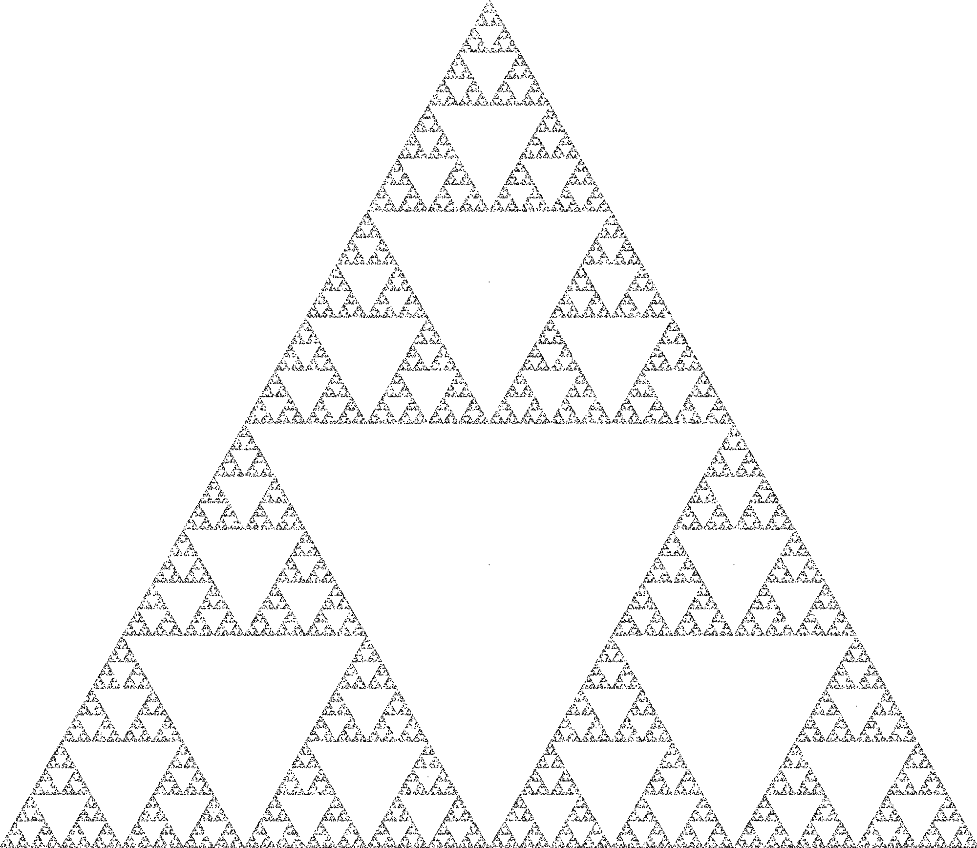
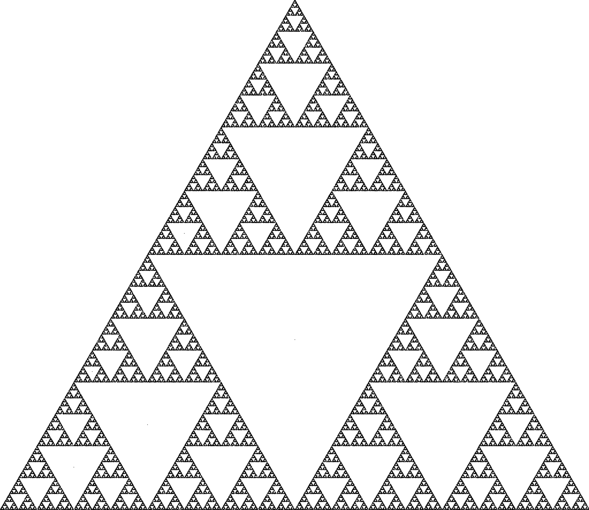
You might expect that the points generated by the chaos game will eventually cover the entire triangle more or less evenly. This is not what happens, however. Figure 1.2 shows the point distributions after 50 000 and 200 000 iterations. As you can see, the points produced by the chaos game are distributed unevenly and converge toward a shape that looks like a triangle from which a number of successively smaller triangles have been cut out. There is a single large empty triangle in the center, which is surrounded by three smaller ones. Each of these smaller triangles is again surrounded by three smaller triangles, and the pattern continues indefinitely. The longer we let the chaos game run, the more closely the resulting set of points approximates this unexpected limiting shape.

(image) (image)

Figure 1.2 Visualization of the first 50 000 and 200 000 points computed by the chaos game. As the number of iteration increases, the point set slowly converges toward a fractal called the Sierpiński triangle.

This curious shape — known as the Sierpiński triangle — is an example of a fractal. Fractals are geometric objects that share two main properties: They have a “fractured” appearance that is irregular but not random, and they can be magnified indefinitely, revealing new details at every level of magnification. In addition, fractals are often self-similar, which means that their parts resemble the shape as a whole. The Sierpiński triangle clearly has all three properties: Its geometric structure isn’t random but it’s also not as regular as a simple polygon or circle, and it can be magnified indefinitely, with new copies of the Sierpiński triangle appearing at every level of magnification.

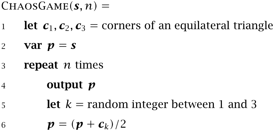
The chaos game we used to construct the Sierpiński triangle is a simple example of an algorithm, a formal description of how to break down a computation into a sequence of elementary steps. To describe algorithms, we will use the format shown in Algorithm 1.1. In this case, the algorithm consists of a single function named ChaosGame that takes two inputs \(\vec {s}\) and \(n\), the starting point and the number of iterations to perform. The numbered lines that follow explain the computational steps performed by the algorithm.

Algorithm 1.1

Given a starting point \(\vec {s}\), produce a sequence of \(n\) points in the plane.

(image)

Let’s take a closer look at the steps of Algorithm 1.1. Line 1 defines three variables \(\vec {c}_1\) to \(\vec {c}_3\) that represent the corners of an equilateral triangle; we assume that these corners are already known or that they are computed using a method not specified in the algorithm. We use the let keyword to define read-only variables that don’t change over the course of the algorithm. Line 2 defines a new variable \(\vec {p}\) for the current position and initializes it to the starting point \(\vec {s}\). This variable is defined using the var keyword, which indicates that the value of \(\vec {p}\) is modified as the algorithm progresses. The repeat loop on the following line repeats the indented lines in its body \(n\) times. It starts with an output statement that outputs the current value of \(\vec {p}\). Line 5 then sets the constant \(k\) to a random integer between 1 and 3, and line 6 moves \(\vec {p}\) toward the \(k\)th corner. The loop is then repeated \(n-1\) more times. Since output is executed \(n\) times, the algorithm produces \(n\) points.

Mathematicians usually distinguish between points and vectors: Points represent locations in space, whereas a vectors represent directions. However, for simple geometric problems in the plane, the two concepts are closely related: Every point \(P\) with coordinates \((x,y)\) can be represented by the position vector \(\vec {p}=\left (\begin {smallmatrix}x\\y\end {smallmatrix}\right )\) that points from the origin to \(P\), and vice versa.

For the geometric problems discussed in this book, we will keep things simple and use points and positions vectors interchangeably. Boldface symbols like \(\vec {p}\) and \(\vec {q}\) are always vectors, and if we say something like “the point \(\vec {s}\),” what we really mean is “the position vector \(\vec {s}\).”

Implementing the Chaos Game

We can now turn to the fun part: implementing the chaos game so that it runs on a real computer and produces real images. In most cases, turning an algorithm into a working program is more complicated than translating it step by step. For instance, we may have to make changes based on the chosen programming language, flesh out details that weren’t specified precisely, or integrate the algorithm with other parts of a larger program. Here are some of the technical details we have to consider when implementing the ChaosGame algorithm:

  • 1. How do we store points and move them?

  • 2. How do we compute the three corners of the outer triangle?

  • 3. How do we create random numbers between 1 and 3?

  • 4. What does it mean to output a point?

Let’s address these questions one by one.

We start by defining a custom data type called Point that allows us to store and compute with points in the plane. What kinds of operations do we require in Point? Obviously, we need a way to construct points at certain positions in the plane, so that we can specify the starting point of the chaos game and the three corners that enclose the fractal. To store a point’s position we use Cartesian coordinates \((x,y)\), which measure the point’s position along the horizontal and vertical axis. The Point type defined in Listing 1.1 stores these coordinates in two fields x and y.

Listing 1.1ch1 / Point

// A point in 2D.
public record Point(double x, double y) {
    // ...
}

To implement the chaos game, we also need a way to move the current point halfway toward one of the triangle’s corners, that is, we need to compute the midpoint of two points. The easiest way to do this is to average their coordinates, as shown here for the points p and q:

Point midPoint = new Point(
        0.5 * (p.x() + q.x()), 0.5 * (p.y() + q.y()));

This is a special case of a more general operation that computes points along the line segment between two arbitrary points \(\vec {p}\) and \(\vec {q}\). In computer graphics, the point that lies some fraction \(t\) between \(\vec {p}\) and \(\vec {q}\) is commonly denoted by \(\lerp (\vec {p}, \vec {q}, t)\).2 Three special cases of this lerp function are worth noting: For \(t=0\) we obtain the first end point \(\vec {p}\), for \(t=1\) the second end point \(\vec {q}\), and for \(t=1/2\) their midpoint. The function is illustrated in Fig. 1.3.

Figure 1.3 The lerp function computes a point that lies on the line segment between two end points.

There are two equivalent formulas for defining the lerp function. The first is obtained by starting at the first point \(\vec {p}\) and then advancing along the line to \(\vec {q}\) by adding the difference vector \(\vec {q}-\vec {p}\) scaled by \(t\):

\begin{equation*} \label {eq:lerp1} \lerp (\vec {p}, \vec {q}, t) = \vec {p} + t (\vec {q}-\vec {p}). \end{equation*}

The second formula has a more algebraic flavor and expresses the lerp function as the weighted average of \(\vec {p}\) and \(\vec {q}\):

\begin{equation} \label {eq:lerp} \lerp (\vec {p}, \vec {q}, t) = (1-t)\vec {p} + t \vec {q}. \end{equation}

Both definitions can be transformed into each other by reorganizing the terms on the right-hand side. Even though the first definition is slightly more intuitive, we will use the second one since it is more symmetrical and slightly easier to generalize to other forms of interpolation; the implementation is shown in Listing 1.2.

Listing 1.2ch1 / Point

// Compute the linear interpolation of two points.
public static Point lerp(Point p, Point q, double fraction) {
    return new Point((1 - fraction) * p.x + fraction * q.x,
            (1 - fraction) * p.y + fraction * q.y);
}

It’s now easy to implement the chaos game itself. The chaosGame() function in Listing 1.3 takes three arguments — a list of corners, a starting point, and the number of iterations that should be performed — and returns the sequence of points it visits as a list of Points. The function first creates a random number generator rng that is used to select one of the corners in each iteration and then allocates a data structure for the return value, in this case an ArrayList of Points.3 The actual algorithm is implemented by the for loop that follows, which stores the current point in points and then moves it towards a randomly chosen corner.

Listing 1.3ch1 / ChaosGame

public static List<Point> chaosGame(List<Point> corners,
        Point start, int iterations) {
    var rng = new Random();
    var points = new ArrayList<Point>(iterations);
    Point p = start;
    for (int i = 0; i < iterations; i++) {
        points.add(p);
        Point c = corners.get(rng.nextInt(corners.size()));
        p = Point.lerp(p, c, 0.5);
    }
    return points;
}

JDK: Random
Point: lerp()

If we want to create an image of the Sierpiński triangle like the one in Fig. 1.2, we have to simulate a few thousand iterations of the chaos game and then draw the resulting points. One way to do this is shown in Listing 1.4. We first construct a large equilateral triangle with a side length of 1000 and then call chaosGame() to compute 50 000 points inside this triangle, using the center of the triangle as the starting point. Finally, we draw each of the resulting points as a small, filled circle. The Graphics2D type used in this listing is the standard interface provided by Java for producing 2D graphics; Exercise 1.7 asks you to complete this program by setting up a suitable instance of Graphics2D.

Listing 1.4ch1 / ChaosGame

public static void drawSierpinski(Graphics2D g) {
    double sideLength = 1000;
    var corners = List.of(
            new Point(0, 0),
            new Point(sideLength, 0),
            new Point(sideLength / 2, sideLength * Math.sqrt(3) / 2));
    Point start = new Point(
            sideLength / 2, sideLength / Math.sqrt(3) / 2);
    List<Point> points = chaosGame(corners, start, 50_000);

    float radius = 0.01f;
    for (Point p : points.subList(50, points.size()))
        g.fill(new Ellipse2D.Double(p.x(), p.y(), radius, radius));
}

JDK: Ellipse2D, Graphics2D, List, Math
ChaosGame: chaosGame()
Point: Point()

You may be wondering why drawSierpinski() removes the first 50 elements of points before drawing them. The reason is that for some starting points the chaos game may require a few iterations to “warm up” and produce points that are sufficiently close to the actual fractal. In the present example, for instance, we start at the center of the triangle, which isn’t part of the Sierpiński triangle. But with every iteration, the point moves closer to the final fractal until it is imperceptibly close. Discarding the first few points produced by the chaos game is enough to get rid of the obvious outliers and obtain clean-looking images.

2 The name “lerp” is a contraction of “linear interpolation.”

3 In Java, an ArrayList is a special type of List, so the code is correct even though the return type of chaosGame() doesn’t match the type of points exactly.

Exercises

Exercise 1.1.Given two points \(\vec {p}\) and \(\vec {q}\), what is the geometric interpretation of \(\lerp (\vec {p}, \vec {q}, -1)\)?

Exercise 1.2.Extend the Point class with a method distance() that computes the distance between two points.

Exercise 1.3. What happens if you place the starting point of the chaos game outside of the triangle defined by the three corners? What happens if you move the corners of the triangle so that it is no longer equilateral?