Exercise 4.5. The Koch snowflake in Fig. 4.9 is a fractal curve that resembles a snowflake. The curve can be defined recursively:
• The order-0 snowflake is an equilateral triangle.
• The order-\(n\) snowflake is obtained from the order-\(n-1\) snowflake by dividing each edge into three parts, and replacing the middle part with the tip of a small triangle.
Write a program that computes the Koch snowflake of arbitrary order \(n\).
Figure 4.9 Construction of the Koch snowflake.
Closest Points on Lines and Bézier Curves
Exercise 4.6.A common problem in graphical applications is to determine the distance between a given point \(\vec {m}\) (for example the
mouse cursor) and certain geometric objects. In this exercise, we consider the distance to lines, line segments, and Bézier curves.
Let’s start with lines. A line that goes through two points \(\vec {a}=(a_x,a_y)\) and \(\vec {b}=(b_x,b_y)\) can be described as a parametric curve of the following form:
The point \(\vec {x}_c\) on this line that is closest to \(\vec {m}\) is the one for which the segment connecting the two points is perpendicular to the line itself:
Equivalently, the vector \(\vec {m}-\vec {x}_c\) must be perpendicular to the direction of the line \(\vec {b}-\vec {a}\), and since two vectors are perpendicular if their dot product is zero, we have the following condition:
a) Plug Eq. (4.7) into Eq. (4.8) and solve for \(t\) to find a formula for the
closest point.
For line segments we can use the same approach with a small modification. The formula for a line segment from \(\vec {a}\) to \(\vec {b}\) is identical to that of a line, but now the parameter is restricted to the interval between 0 and 1:
To find the closest point on the line segment to a point \(\vec {m}\), we first compute the parameter \(t\) of the closest point along the line through \(\vec {a}\) and \(\vec {b}\), as above. If the resulting parameter satisfies \(0\le t\le 1\), the corresponding point \(\vec {x}_c\) lies
on the line segment and is the desired closest point. Otherwise, if \(t<0\) or \(t>1\), the closest point is one of the end points \(\vec {a}\) or \(\vec {b}\).
b) Write a class LineSegment that represents a line segment between two Points. Define the following two methods:
Point pointAt(double t);
Point closestPoint(Point m);
The first method pointAt() implements Eq. (4.9) and returns the point corresponding to a given parameter t. The second method closestPoint() computes the closest point to m on the line segment.
Finding the closest point on a Bézier curve is more difficult. While it is possible to derive a mathematical criterion similar to Eq. (4.8), the resulting equation is a quintic (order 5) polynomial
in \(t\) that cannot be solved analytically. But if we are content with an approximate result, we can find the closest point to \(\vec {m}\) by subdividing the curve into line segments, finding the closest point on each, and returning the overall minimum.
c) Devise a recursive algorithm for computing the point on a Bézier curve that is closest to a given point \(\vec {m}\) by extending de Casteljau’s algorithm.
Bézier Curves Continued
Exercise 4.7.As we saw in the text, cubic Bézier curves can be constructed by repeatedly averaging four given control points using de Casteljau’s
algorithm. If we start with a different number of control points, we obtain Bézier curves of a different order. In particular, if we start three control points \(\vec {p}_0\), \(\vec {p}_1\), and \(\vec {p}_2\), de Casteljau’s algorithm produces a quadratic Bézier curve. An example of a quadratic Bézier curve is shown in Fig. 4.10.
Figure 4.10 A quadratic Bézier curve. When starting with only three control points, de Casteljau’s algorithm produces a point on a quadratic Bézier curve.
a) Show that the construction produces a point that lies on the curve
b) Devise a criterion for determining whether a quadratic Bézier curve is approximately straight.
c) Develop a recursive algorithm for adaptively subdividing quadratic Bézier curves.
\(\star \) Exercise 4.8. In the text we stated and used a few properties of Bézier curves without proof, most importantly the relationship between the parametric form of Bézier
curves in Eq. (4.2) and de Casteljau’s algorithm.
a) Show that de Casteljau’s method shown in Fig. 4.6 yields the point \(\vec {B}(1/2)\) on the Bézier curve.
b) Use a similar derivation to show that any point \(\vec {B}(t)\) can be computed by starting with \(\vec {p}_0, \dots , \vec {p}_3\) and repeatedly combining adjacent points \(\vec {a},\vec {b}\) using \(\lerp (\vec {a}, \vec {b}, t)\).
c) Show that a Bézier curve whose two control points are placed \(1/3\) and \(2/3\) of the way between its two end points is a line segment.
d) Given an affine transformation \(A(\vec {x})=\vec {A}\vec {x}+\vec {a}\) and a Bézier curve \(\vec {B}(t)\) specified by four control points \(\vec {p}_0,\dots ,\vec {p}_3\), show that the transformed Bézier curve \(\vec {B}'(t)=A(\vec {B}(t))\) is equal
to the Bézier curve that corresponds to the transformed control points \(\vec {p}_k'=A(\vec {p}_k)\). (What this means is that Bézier curves can be rotated, scaled, and sheared simply by transforming their control points.) Hint: Use Eq. (4.4).
Penrose Tilings
Exercise 4.9.An arrangement of shapes that covers a surface seamlessly and without overlap is called a tiling or a tessellation. The simplest tilings — commonly used in bathrooms and board games — use regular polygons such as triangles, squares, or hexagons to cover the plane. A famous example of a more complicated tiling is the Penrose tiling shown in Fig. 4.11.
Figure 4.11 Example of a Penrose tiling. Penrose tilings seamlessly cover the plane with two kinds of rhombs that are arranged according to specific rules. It can be shown that Penrose tilings are aperiodic: on a global scale, the arrangement of rhombs never
exactly repeats itself.
Penrose tilings consist of two different shapes, a thick rhomb whose inner angles are \(72\) and \(108\) degrees and a thin rhomb whose inner angles are \(36\) and \(144\) degrees:
To obtain a valid Penrose tiling, these two kinds of rhombs must be placed in such a way that the arrow symbols on all shared edges point in the same direction and have the same number of arrow heads. It’s these placement rules that give Penrose tilings their many fascinating properties. For instance, it
can be shown that it is possible to cover the entire plane with Penrose tiles and that the resulting pattern is always aperiodic — it extends indefinitely but never repeats itself.1
a) One recurring pattern in Fig. 4.11 is a five-pointed star that consists of five thick rhombs. In such a star, do the arrows on the shared edges point inwards or outwards? Is it possible to build a similar star out of
ten thin rhombs?
An important property of Penrose tilings is that they can be subdivided recursively: Given any legal arrangement of Penrose tiles, it is possible to split and reassemble the rhombs in such a way that the result is again a valid arrangement of smaller tiles. This process is known as deflation since it decreases the size of the rhombs.
The deflation rules are illustrated in Fig. 4.12. First, we split each rhomb into two triangles that are mirror images of each other and mark the common edge with a new arrow symbol that allows us to later reassemble the triangles
into rhombs. We then subdivide each triangle into multiple smaller triangles as shown in the bottom part of the figure. This subdivision splits existing edges according to the golden ratio \(1:\bigl (1+\sqrt {5}\bigr )/2\). Notice that each new triangle is a scaled-down version of one of the original triangles.
.
Figure 4.12 Subdivision rules for Penrose tilings. Each rhomb is first split into two triangles, which are then further subdivided into smaller triangles of the same shape.
You can convince yourself that this subdivision scheme is consistent with the rules for Penrose tilings. For example, every outer edge with a single arrow “\(\rangle \)” is transformed into two edges, one with three reversed arrows “\(\langle \langle \langle \)” and one with two reversed
arrows “\(\langle \langle \)”. We can therefore take any valid arrangement of rhombs, perform any number of subdivision steps, and obtain an arrangement of triangles that can be recombined into a valid Penrose tiling. (The only exception are triangles that lie on the boundary, which may not
have a counterpart to combine with.)
b) Sketch the result of deflating a thick rhomb twice; in other words, extend the left part of Fig. 4.12 with a second subdivision step. How many complete rhombs do you get?
The deflation process can be repeated multiple times, each time producing a more detailed tiling. The tiling shown in Fig. 4.11, for example, was obtained by starting with a single thick rhomb (the outline of the tiling) and deflating it seven
times.
c) Write a program for deflating thick and thin rhombs a given number of times. Hint: It is easier to work with triangles instead of rhombs.
1 A good way to experiment with Penrose tilings is to craft a small stack of rhombs out of paper; the required ratio of thick to thin rhombs is approximately \(1.6:1\). Alternatively, an interactive web page by Kevin Bertman for experimenting with Penrose tilings can be found at
http://www.mrbertman.com/penroseTilings.html.
Plotting Parametric Curves
Exercise 4.10.A parametric curve is a function that maps an interval of real numbers \([a,b]\) to points in the plane; the parametric form
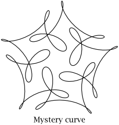
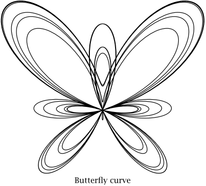
of Bézier curves in Eq. (4.2) is an example of a parametric curve. Figure 4.13 shows two examples of more complicated parametric curves. The
first is the so-called “mystery curve” which owes its name to its unexpected five-fold symmetry.2 Its shape is described by the following formula:
As the parameter \(t\) goes through the range \(0\le t\le 2\pi \), the points \(\vec {C}(t)\) continuously trace out the left curve in the figure. The other curve is the “Butterfly curve,” which is described by the following formula:
(The notation \(\sin ^5x\) is a shorthand for \((\sin x)^5\).)
Figure 4.13 Examples of two-dimensional parametric curves.
a) Design an interface for representing and evaluating parametric curves and use it to implement the mystery curve.
To draw a given parametric curve \(\vec {C}(t)\), we compute a sequence of points \(\vec {p}_1,\dots ,\vec {p}_N\) on the curve and connect them using line segments. Each point \(\vec {p}_k\) is obtained by evaluating the parametric curve at a certain parameter \(t_k\) so that \(\vec
{p}_k = C(t_k)\).
The main challenge is to place the points \(\vec {p}_k\) in such a way that connecting them using line segments produces a reasonably accurate image of the curve. As in our discussion of Bézier curves, the simplest approach is to divide the parameter range \([a,b]\) into \(N\) pieces of the same
size, which gives us \(t_k = (b-a)/N\) or
The only parameter in this case is the number \(N\) of line segments.
b) Experiment with drawing the mystery and butterfly curves. How large do you have to choose \(N\) in each case to obtain a reasonably smooth rendition of the curve?
As in our discussion of Bézier curves, there are two main problems with rigid subdivision schemes like this: They provide no control over the placement of points along the curve, and choosing a suitable number of line segments requires a lot of trial and error. A better solution is to perform the subdivision
adaptively, by repeatedly splitting curve segments into smallers parts until they are straight enough to be replaced by line segments. Splitting a parametric curve is easily done by splitting its parameter range: If the current parameter range is \(a\le t<b\), we
split it into two halves \(a \le t<(a+b)/2\) and \((a+b)/2\le t < b\).
Unfortunately, there is no reliable way to measure the straightness of a general parametric curve since we have no a priori knowledge about the shape of the curve. The best we can do is devise a straightness test that works well for smooth curves and fails gracefully for curves that aren’t well-behaved.
c) Given a parametric curve \(\vec {C}(t)\) and a parameter range \([a,b]\), suggest a simple heuristic that decides whether the curve segment between \(\vec {C}(a)\) and \(\vec {C}(b)\) is relatively straight.
d) Write a program that plots a parametric curve for a given parameter range. The algorithm should adaptively subdivide the parameter range until all curve segments are almost straight. What parameters does your algorithm have? How do you
ensure that it always terminates?
e) Use your algorithm to draw the mystery curve and the Butterfly curve. Compare the resulting curves to those you obtained in part (b).
Here are the formulas of two additional parametric curves that you can use for testing:
\(\seteqnumber{0}{4.}{12}\)
\begin{align*}
\vec {C}(t) &= \begin{pmatrix} A\cos (at + \delta )\\ B\sin (bt) \end {pmatrix} && \text {Lissajous curve}\\ \vec {C}(t) &= \begin{pmatrix} A\cos (at) \cos (t)\\ A\cos (at) \sin (t) \end {pmatrix} && \text {Rhodonea curve}
\end{align*}
As usual, \(t\) is the curve parameter, and \(A, a, B, b, \delta \) are additional parameters that determine the shape of the curve.
2 For a detailed discussion of the mystery curve and its symmetry, see [36].