☰

1 Iterated Function Systems

\(\newcommand{\footnotename}{footnote}\) \(\def \LWRfootnote {1}\) \(\newcommand {\footnote }[2][\LWRfootnote ]{{}^{\mathrm {#1}}}\) \(\newcommand {\footnotemark }[1][\LWRfootnote ]{{}^{\mathrm {#1}}}\) \(\let \LWRorighspace \hspace \) \(\renewcommand {\hspace }{\ifstar \LWRorighspace \LWRorighspace }\) \(\newcommand {\TextOrMath }[2]{#2}\) \(\newcommand {\mathnormal }[1]{{#1}}\) \(\newcommand \ensuremath [1]{#1}\) \(\newcommand {\LWRframebox }[2][]{\fbox {#2}} \newcommand {\framebox }[1][]{\LWRframebox } \) \(\newcommand {\setlength }[2]{}\) \(\newcommand {\addtolength }[2]{}\) \(\newcommand {\setcounter }[2]{}\) \(\newcommand {\addtocounter }[2]{}\) \(\newcommand {\arabic }[1]{}\) \(\newcommand {\number }[1]{}\) \(\newcommand {\noalign }[1]{\text {#1}\notag \\}\) \(\newcommand {\cline }[1]{}\) \(\newcommand {\directlua }[1]{\text {(directlua)}}\) \(\newcommand {\luatexdirectlua }[1]{\text {(directlua)}}\) \(\newcommand {\protect }{}\) \(\def \LWRabsorbnumber #1 {}\) \(\def \LWRabsorbquotenumber "#1 {}\) \(\newcommand {\LWRabsorboption }[1][]{}\) \(\newcommand {\LWRabsorbtwooptions }[1][]{\LWRabsorboption }\) \(\def \mathchar {\ifnextchar "\LWRabsorbquotenumber \LWRabsorbnumber }\) \(\def \mathcode #1={\mathchar }\) \(\let \delcode \mathcode \) \(\let \delimiter \mathchar \) \(\def \oe {\unicode {x0153}}\) \(\def \OE {\unicode {x0152}}\) \(\def \ae {\unicode {x00E6}}\) \(\def \AE {\unicode {x00C6}}\) \(\def \aa {\unicode {x00E5}}\) \(\def \AA {\unicode {x00C5}}\) \(\def \o {\unicode {x00F8}}\) \(\def \O {\unicode {x00D8}}\) \(\def \l {\unicode {x0142}}\) \(\def \L {\unicode {x0141}}\) \(\def \ss {\unicode {x00DF}}\) \(\def \SS {\unicode {x1E9E}}\) \(\def \dag {\unicode {x2020}}\) \(\def \ddag {\unicode {x2021}}\) \(\def \P {\unicode {x00B6}}\) \(\def \copyright {\unicode {x00A9}}\) \(\def \pounds {\unicode {x00A3}}\) \(\let \LWRref \ref \) \(\renewcommand {\ref }{\ifstar \LWRref \LWRref }\) \( \newcommand {\multicolumn }[3]{#3}\) \(\require {textcomp}\) \(\newcommand {\intertext }[1]{\text {#1}\notag \\}\) \(\let \Hat \hat \) \(\let \Check \check \) \(\let \Tilde \tilde \) \(\let \Acute \acute \) \(\let \Grave \grave \) \(\let \Dot \dot \) \(\let \Ddot \ddot \) \(\let \Breve \breve \) \(\let \Bar \bar \) \(\let \Vec \vec \) \(\renewcommand {\vec }{\boldsymbol }\) \(\newcommand {\Edge }{\ensuremath {\,\textemdash \,}}\) \(\newcommand \Const [1]{\text {\textsf {#1}}}\) \(\DeclareMathOperator {\lerp }{lerp}\) \(\DeclareMathOperator {\bitlen }{bitlen}\) \(\DeclareMathOperator {\sign }{sign}\) \(\newcommand {\I }{\mathrm {i}}\) \(\newcommand \AND {\mathbin {\&}}\) \(\newcommand \OR {\mathbin {|}}\) \(\newcommand \XOR {\mathbin {{}^{\wedge }}}\) \(\newcommand \shl {\ll }\) \(\newcommand \shr {\ggg }\) \(\newcommand \asr {\gg }\) \(\newcommand \NOT {\ensuremath {\mathord {\sim }}}\) \(\newcommand {\isep }{\mathrel {{.}\,{.}}}\) \(\newcommand {\Id }[1]{\mathit {#1}}\) \(\newcommand {\const }[1]{\mathsf {#1}}\) \(\newcommand {\algorithmname }[1]{\text {\textsc {#1}}}\) \(\newcommand {\bits }[1]{\text {#1}}\) \(\newcommand {\hexa }[1]{\mathtt {0x#1}}\) \(\newcommand {\num }[1]{#1}\) \(\newcommand {\qed }{\quad \square }\) \(\newcommand {\idiv }[2]{\lfloor #1/#2\rfloor }\) \(\newcommand \attribdot {\ensuremath {\mkern 1.5mu.\mkern 1.5mu}}\) \(\newcommand \attribxr [2]{#1\attribdot \text {#2}}\) \(\newcommand \attribir [2]{\Id {#1}\attribdot \text {#2}}\) \(\newcommand \attribii [2]{\Id {#1}\attribdot \Id {#2}}\) \(\newcommand \textsc [1]{#1}\) \(\require {colortbl}\) \(\let \LWRorigcolumncolor \columncolor \) \(\renewcommand {\columncolor }[2][named]{\LWRorigcolumncolor [#1]{#2}\LWRabsorbtwooptions }\) \(\let \LWRorigrowcolor \rowcolor \) \(\renewcommand {\rowcolor }[2][named]{\LWRorigrowcolor [#1]{#2}\LWRabsorbtwooptions }\) \(\let \LWRorigcellcolor \cellcolor \) \(\renewcommand {\cellcolor }[2][named]{\LWRorigcellcolor [#1]{#2}\LWRabsorbtwooptions }\) \(\newcommand {\tcbset }[1]{}\) \(\newcommand {\tcbsetforeverylayer }[1]{}\) \(\newcommand {\tcbox }[2][]{\boxed {\text {#2}}}\) \(\newcommand {\tcboxfit }[2][]{\boxed {#2}}\) \(\newcommand {\tcblower }{}\) \(\newcommand {\tcbline }{}\) \(\newcommand {\tcbtitle }{}\) \(\newcommand {\tcbsubtitle [2][]{\mathrm {#2}}}\) \(\newcommand {\tcboxmath }[2][]{\boxed {#2}}\) \(\newcommand {\tcbhighmath }[2][]{\boxed {#2}}\) \(\newcommand {\toprule }[1][]{\hline }\) \(\let \midrule \toprule \) \(\let \bottomrule \toprule \) \(\def \LWRbooktabscmidruleparen (#1)#2{}\) \(\newcommand {\LWRbooktabscmidrulenoparen }[1]{}\) \(\newcommand {\cmidrule }[1][]{\ifnextchar (\LWRbooktabscmidruleparen \LWRbooktabscmidrulenoparen }\) \(\newcommand {\morecmidrules }{}\) \(\newcommand {\specialrule }[3]{\hline }\) \(\newcommand {\addlinespace }[1][]{}\) \(\newcommand {\LWRsubmultirow }[2][]{#2}\) \(\newcommand {\LWRmultirow }[2][]{\LWRsubmultirow }\) \(\newcommand {\multirow }[2][]{\LWRmultirow }\) \(\newcommand {\mrowcell }{}\) \(\newcommand {\mcolrowcell }{}\) \(\newcommand {\STneed }[1]{}\) \(\newcommand {\LWRldelimtwo }[1][]{\text {#1}~\LWRbigdelim }\) \(\newcommand {\LWRldelimone }[2][]{\LWRldelimtwo }\) \(\def \ldelim #1#2{\def \LWRbigdelim {#1}\LWRldelimone }\) \(\newcommand {\LWRrdelimtwo }[1][]{\LWRbigdelim ~\text {#1}}\) \(\newcommand {\LWRrdelimone }[2][]{\LWRrdelimtwo }\) \(\def \rdelim #1#2{\def \LWRbigdelim {#1}\LWRrdelimone }\) \(\let \symnormal \mathit \) \(\let \symliteral \mathrm \) \(\let \symbb \mathbb \) \(\let \symbbit \mathbb \) \(\let \symcal \mathcal \) \(\let \symscr \mathscr \) \(\let \symfrak \mathfrak \) \(\let \symsfup \mathsf \) \(\let \symsfit \mathit \) \(\let \symbfsf \mathbf \) \(\let \symbfup \mathbf \) \(\newcommand {\symbfit }[1]{\boldsymbol {#1}}\) \(\let \symbfcal \mathcal \) \(\let \symbfscr \mathscr \) \(\let \symbffrak \mathfrak \) \(\let \symbfsfup \mathbf \) \(\newcommand {\symbfsfit }[1]{\boldsymbol {#1}}\) \(\let \symup \mathrm \) \(\let \symbf \mathbf \) \(\let \symit \mathit \) \(\let \symsf \symsfit \) \(\let \symtt \mathtt \) \(\let \symbffrac \mathbffrac \) \(\newcommand {\mathfence }[1]{\mathord {#1}}\) \(\newcommand {\mathover }[1]{#1}\) \(\newcommand {\mathunder }[1]{#1}\) \(\newcommand {\mathaccent }[1]{#1}\) \(\newcommand {\mathbotaccent }[1]{#1}\) \(\newcommand {\mathalpha }[1]{\mathord {#1}}\) \(\def\Alpha{\unicode{x1D6E2}}\) \(\def\Beta{\unicode{x1D6E3}}\) \(\def\Gamma{\unicode{x1D6E4}}\) \(\def\Digamma{\mathit{\unicode{x03DC}}}\) \(\def\Delta{\unicode{x1D6E5}}\) \(\def\Epsilon{\unicode{x1D6E6}}\) \(\def\Zeta{\unicode{x1D6E7}}\) \(\def\Eta{\unicode{x1D6E8}}\) \(\def\Theta{\unicode{x1D6E9}}\) \(\def\Vartheta{\unicode{x1D6F3}}\) \(\def\Iota{\unicode{x1D6EA}}\) \(\def\Kappa{\unicode{x1D6EB}}\) \(\def\Lambda{\unicode{x1D6EC}}\) \(\def\Mu{\unicode{x1D6ED}}\) \(\def\Nu{\unicode{x1D6EE}}\) \(\def\Xi{\unicode{x1D6EF}}\) \(\def\Omicron{\unicode{x1D6F0}}\) \(\def\Pi{\unicode{x1D6F1}}\) \(\def\Rho{\unicode{x1D6F2}}\) \(\def\Sigma{\unicode{x1D6F4}}\) \(\def\Tau{\unicode{x1D6F5}}\) \(\def\Upsilon{\unicode{x1D6F6}}\) \(\def\Phi{\unicode{x1D6F7}}\) \(\def\Chi{\unicode{x1D6F8}}\) \(\def\Psi{\unicode{x1D6F9}}\) \(\def\Omega{\unicode{x1D6FA}}\) \(\def\alpha{\unicode{x1D6FC}}\) \(\def\beta{\unicode{x1D6FD}}\) \(\def\varbeta{\unicode{x03D0}}\) \(\def\gamma{\unicode{x1D6FE}}\) \(\def\digamma{\mathit{\unicode{x03DD}}}\) \(\def\delta{\unicode{x1D6FF}}\) \(\def\epsilon{\unicode{x1D716}}\) \(\def\varepsilon{\unicode{x1D700}}\) \(\def\zeta{\unicode{x1D701}}\) \(\def\eta{\unicode{x1D702}}\) \(\def\theta{\unicode{x1D703}}\) \(\def\vartheta{\unicode{x1D717}}\) \(\def\iota{\unicode{x1D704}}\) \(\def\kappa{\unicode{x1D705}}\) \(\def\varkappa{\unicode{x1D718}}\) \(\def\lambda{\unicode{x1D706}}\) \(\def\mu{\unicode{x1D707}}\) \(\def\nu{\unicode{x1D708}}\) \(\def\xi{\unicode{x1D709}}\) \(\def\omicron{\unicode{x1D70A}}\) \(\def\pi{\unicode{x1D70B}}\) \(\def\varpi{\unicode{x1D71B}}\) \(\def\rho{\unicode{x1D70C}}\) \(\def\varrho{\unicode{x1D71A}}\) \(\def\sigma{\unicode{x1D70E}}\) \(\def\varsigma{\unicode{x1D70D}}\) \(\def\tau{\unicode{x1D70F}}\) \(\def\upsilon{\unicode{x1D710}}\) \(\def\phi{\unicode{x1D719}}\) \(\def\varphi{\unicode{x1D711}}\) \(\def\chi{\unicode{x1D712}}\) \(\def\psi{\unicode{x1D713}}\) \(\def\omega{\unicode{x1D714}}\) \(\def\upAlpha{\unicode{x0391}}\) \(\def\upBeta{\unicode{x0392}}\) \(\def\upGamma{\unicode{x0393}}\) \(\def\upDigamma{\unicode{x03DC}}\) \(\def\upDelta{\unicode{x0394}}\) \(\def\upEpsilon{\unicode{x0395}}\) \(\def\upZeta{\unicode{x0396}}\) \(\def\upEta{\unicode{x0397}}\) \(\def\upTheta{\unicode{x0398}}\) \(\def\upVartheta{\unicode{x03F4}}\) \(\def\upIota{\unicode{x0399}}\) \(\def\upKappa{\unicode{x039A}}\) \(\def\upLambda{\unicode{x039B}}\) \(\def\upMu{\unicode{x039C}}\) \(\def\upNu{\unicode{x039D}}\) \(\def\upXi{\unicode{x039E}}\) \(\def\upOmicron{\unicode{x039F}}\) \(\def\upPi{\unicode{x03A0}}\) \(\def\upVarpi{\unicode{x03D6}}\) \(\def\upRho{\unicode{x03A1}}\) \(\def\upSigma{\unicode{x03A3}}\) \(\def\upTau{\unicode{x03A4}}\) \(\def\upUpsilon{\unicode{x03A5}}\) \(\def\upPhi{\unicode{x03A6}}\) \(\def\upChi{\unicode{x03A7}}\) \(\def\upPsi{\unicode{x03A8}}\) \(\def\upOmega{\unicode{x03A9}}\) \(\def\itAlpha{\unicode{x1D6E2}}\) \(\def\itBeta{\unicode{x1D6E3}}\) \(\def\itGamma{\unicode{x1D6E4}}\) \(\def\itDigamma{\mathit{\unicode{x03DC}}}\) \(\def\itDelta{\unicode{x1D6E5}}\) \(\def\itEpsilon{\unicode{x1D6E6}}\) \(\def\itZeta{\unicode{x1D6E7}}\) \(\def\itEta{\unicode{x1D6E8}}\) \(\def\itTheta{\unicode{x1D6E9}}\) \(\def\itVartheta{\unicode{x1D6F3}}\) \(\def\itIota{\unicode{x1D6EA}}\) \(\def\itKappa{\unicode{x1D6EB}}\) \(\def\itLambda{\unicode{x1D6EC}}\) \(\def\itMu{\unicode{x1D6ED}}\) \(\def\itNu{\unicode{x1D6EE}}\) \(\def\itXi{\unicode{x1D6EF}}\) \(\def\itOmicron{\unicode{x1D6F0}}\) \(\def\itPi{\unicode{x1D6F1}}\) \(\def\itRho{\unicode{x1D6F2}}\) \(\def\itSigma{\unicode{x1D6F4}}\) \(\def\itTau{\unicode{x1D6F5}}\) \(\def\itUpsilon{\unicode{x1D6F6}}\) \(\def\itPhi{\unicode{x1D6F7}}\) \(\def\itChi{\unicode{x1D6F8}}\) \(\def\itPsi{\unicode{x1D6F9}}\) \(\def\itOmega{\unicode{x1D6FA}}\) \(\def\upalpha{\unicode{x03B1}}\) \(\def\upbeta{\unicode{x03B2}}\) \(\def\upvarbeta{\unicode{x03D0}}\) \(\def\upgamma{\unicode{x03B3}}\) \(\def\updigamma{\unicode{x03DD}}\) \(\def\updelta{\unicode{x03B4}}\) \(\def\upepsilon{\unicode{x03F5}}\) \(\def\upvarepsilon{\unicode{x03B5}}\) \(\def\upzeta{\unicode{x03B6}}\) \(\def\upeta{\unicode{x03B7}}\) \(\def\uptheta{\unicode{x03B8}}\) \(\def\upvartheta{\unicode{x03D1}}\) \(\def\upiota{\unicode{x03B9}}\) \(\def\upkappa{\unicode{x03BA}}\) \(\def\upvarkappa{\unicode{x03F0}}\) \(\def\uplambda{\unicode{x03BB}}\) \(\def\upmu{\unicode{x03BC}}\) \(\def\upnu{\unicode{x03BD}}\) \(\def\upxi{\unicode{x03BE}}\) \(\def\upomicron{\unicode{x03BF}}\) \(\def\uppi{\unicode{x03C0}}\) \(\def\upvarpi{\unicode{x03D6}}\) \(\def\uprho{\unicode{x03C1}}\) \(\def\upvarrho{\unicode{x03F1}}\) \(\def\upsigma{\unicode{x03C3}}\) \(\def\upvarsigma{\unicode{x03C2}}\) \(\def\uptau{\unicode{x03C4}}\) \(\def\upupsilon{\unicode{x03C5}}\) \(\def\upphi{\unicode{x03D5}}\) \(\def\upvarphi{\unicode{x03C6}}\) \(\def\upchi{\unicode{x03C7}}\) \(\def\uppsi{\unicode{x03C8}}\) \(\def\upomega{\unicode{x03C9}}\) \(\def\italpha{\unicode{x1D6FC}}\) \(\def\itbeta{\unicode{x1D6FD}}\) \(\def\itvarbeta{\unicode{x03D0}}\) \(\def\itgamma{\unicode{x1D6FE}}\) \(\def\itdigamma{\mathit{\unicode{x03DD}}}\) \(\def\itdelta{\unicode{x1D6FF}}\) \(\def\itepsilon{\unicode{x1D716}}\) \(\def\itvarepsilon{\unicode{x1D700}}\) \(\def\itzeta{\unicode{x1D701}}\) \(\def\iteta{\unicode{x1D702}}\) \(\def\ittheta{\unicode{x1D703}}\) \(\def\itvartheta{\unicode{x1D717}}\) \(\def\itiota{\unicode{x1D704}}\) \(\def\itkappa{\unicode{x1D705}}\) \(\def\itvarkappa{\unicode{x1D718}}\) \(\def\itlambda{\unicode{x1D706}}\) \(\def\itmu{\unicode{x1D707}}\) \(\def\itnu{\unicode{x1D708}}\) \(\def\itxi{\unicode{x1D709}}\) \(\def\itomicron{\unicode{x1D70A}}\) \(\def\itpi{\unicode{x1D70B}}\) \(\def\itvarpi{\unicode{x1D71B}}\) \(\def\itrho{\unicode{x1D70C}}\) \(\def\itvarrho{\unicode{x1D71A}}\) \(\def\itsigma{\unicode{x1D70E}}\) \(\def\itvarsigma{\unicode{x1D70D}}\) \(\def\ittau{\unicode{x1D70F}}\) \(\def\itupsilon{\unicode{x1D710}}\) \(\def\itphi{\unicode{x1D719}}\) \(\def\itvarphi{\unicode{x1D711}}\) \(\def\itchi{\unicode{x1D712}}\) \(\def\itpsi{\unicode{x1D713}}\) \(\def\itomega{\unicode{x1D714}}\) \(\let \lparen (\) \(\let \rparen )\) \(\newcommand {\cuberoot }[1]{\,{}^3\!\!\sqrt {#1}}\,\) \(\newcommand {\fourthroot }[1]{\,{}^4\!\!\sqrt {#1}}\,\) \(\newcommand {\longdivision }[1]{\mathord {\unicode {x027CC}#1}}\) \(\newcommand {\mathcomma }{,}\) \(\newcommand {\mathcolon }{:}\) \(\newcommand {\mathsemicolon }{;}\) \(\newcommand {\overbracket }[1]{\mathinner {\overline {\ulcorner {#1}\urcorner }}}\) \(\newcommand {\underbracket }[1]{\mathinner {\underline {\llcorner {#1}\lrcorner }}}\) \(\newcommand {\overbar }[1]{\mathord {#1\unicode {x00305}}}\) \(\newcommand {\ovhook }[1]{\mathord {#1\unicode {x00309}}}\) \(\newcommand {\ocirc }[1]{\mathord {#1\unicode {x0030A}}}\) \(\newcommand {\candra }[1]{\mathord {#1\unicode {x00310}}}\) \(\newcommand {\oturnedcomma }[1]{\mathord {#1\unicode {x00312}}}\) \(\newcommand {\ocommatopright }[1]{\mathord {#1\unicode {x00315}}}\) \(\newcommand {\droang }[1]{\mathord {#1\unicode {x0031A}}}\) \(\newcommand {\leftharpoonaccent }[1]{\mathord {#1\unicode {x020D0}}}\) \(\newcommand {\rightharpoonaccent }[1]{\mathord {#1\unicode {x020D1}}}\) \(\newcommand {\vertoverlay }[1]{\mathord {#1\unicode {x020D2}}}\) \(\newcommand {\leftarrowaccent }[1]{\mathord {#1\unicode {x020D0}}}\) \(\newcommand {\annuity }[1]{\mathord {#1\unicode {x020E7}}}\) \(\newcommand {\widebridgeabove }[1]{\mathord {#1\unicode {x020E9}}}\) \(\newcommand {\asteraccent }[1]{\mathord {#1\unicode {x020F0}}}\) \(\newcommand {\threeunderdot }[1]{\mathord {#1\unicode {x020E8}}}\) \(\newcommand {\Bbbsum }{\mathop {\unicode {x2140}}\limits }\) \(\newcommand {\oiint }{\mathop {\unicode {x222F}}\limits }\) \(\newcommand {\oiiint }{\mathop {\unicode {x2230}}\limits }\) \(\newcommand {\intclockwise }{\mathop {\unicode {x2231}}\limits }\) \(\newcommand {\ointclockwise }{\mathop {\unicode {x2232}}\limits }\) \(\newcommand {\ointctrclockwise }{\mathop {\unicode {x2233}}\limits }\) \(\newcommand {\varointclockwise }{\mathop {\unicode {x2232}}\limits }\) \(\newcommand {\leftouterjoin }{\mathop {\unicode {x27D5}}\limits }\) \(\newcommand {\rightouterjoin }{\mathop {\unicode {x27D6}}\limits }\) \(\newcommand {\fullouterjoin }{\mathop {\unicode {x27D7}}\limits }\) \(\newcommand {\bigbot }{\mathop {\unicode {x27D8}}\limits }\) \(\newcommand {\bigtop }{\mathop {\unicode {x27D9}}\limits }\) \(\newcommand {\xsol }{\mathop {\unicode {x29F8}}\limits }\) \(\newcommand {\xbsol }{\mathop {\unicode {x29F9}}\limits }\) \(\newcommand {\bigcupdot }{\mathop {\unicode {x2A03}}\limits }\) \(\newcommand {\bigsqcap }{\mathop {\unicode {x2A05}}\limits }\) \(\newcommand {\conjquant }{\mathop {\unicode {x2A07}}\limits }\) \(\newcommand {\disjquant }{\mathop {\unicode {x2A08}}\limits }\) \(\newcommand {\bigtimes }{\mathop {\unicode {x2A09}}\limits }\) \(\newcommand {\modtwosum }{\mathop {\unicode {x2A0A}}\limits }\) \(\newcommand {\sumint }{\mathop {\unicode {x2A0B}}\limits }\) \(\newcommand {\intbar }{\mathop {\unicode {x2A0D}}\limits }\) \(\newcommand {\intBar }{\mathop {\unicode {x2A0E}}\limits }\) \(\newcommand {\fint }{\mathop {\unicode {x2A0F}}\limits }\) \(\newcommand {\cirfnint }{\mathop {\unicode {x2A10}}\limits }\) \(\newcommand {\awint }{\mathop {\unicode {x2A11}}\limits }\) \(\newcommand {\rppolint }{\mathop {\unicode {x2A12}}\limits }\) \(\newcommand {\scpolint }{\mathop {\unicode {x2A13}}\limits }\) \(\newcommand {\npolint }{\mathop {\unicode {x2A14}}\limits }\) \(\newcommand {\pointint }{\mathop {\unicode {x2A15}}\limits }\) \(\newcommand {\sqint }{\mathop {\unicode {x2A16}}\limits }\) \(\newcommand {\intlarhk }{\mathop {\unicode {x2A17}}\limits }\) \(\newcommand {\intx }{\mathop {\unicode {x2A18}}\limits }\) \(\newcommand {\intcap }{\mathop {\unicode {x2A19}}\limits }\) \(\newcommand {\intcup }{\mathop {\unicode {x2A1A}}\limits }\) \(\newcommand {\upint }{\mathop {\unicode {x2A1B}}\limits }\) \(\newcommand {\lowint }{\mathop {\unicode {x2A1C}}\limits }\) \(\newcommand {\bigtriangleleft }{\mathop {\unicode {x2A1E}}\limits }\) \(\newcommand {\zcmp }{\mathop {\unicode {x2A1F}}\limits }\) \(\newcommand {\zpipe }{\mathop {\unicode {x2A20}}\limits }\) \(\newcommand {\zproject }{\mathop {\unicode {x2A21}}\limits }\) \(\newcommand {\biginterleave }{\mathop {\unicode {x2AFC}}\limits }\) \(\newcommand {\bigtalloblong }{\mathop {\unicode {x2AFF}}\limits }\) \(\newcommand {\arabicmaj }{\mathop {\unicode {x1EEF0}}\limits }\) \(\newcommand {\arabichad }{\mathop {\unicode {x1EEF1}}\limits }\)

1.2 Generalizing the Chaos Game

The chaos game as we have discussed it in the previous section can be generalized to a more powerful algorithm for generating fractals. As before, we simulate the movement of a point in the plane, but instead of moving the point toward a randomly chosen corner of a triangle, we instead transform it using a randomly chosen function. For reasons we will explain in a moment, we usually associate with each function \(f_k\) a probability \(p_k\), which determines how frequently the chaos game chooses this function relative to the others. We call the combination of functions and their probabilities an iterated function system or IFS.

It’s easy to see that this is a proper generalization: If \(\vec {c}_1, \vec {c}_2, \vec {c}_3\) are the corners of a triangle, we can define three functions that move a given point \(\vec {p}\) halfway toward each of the corners:

\begin{equation*} f_1(\vec {p}) = (\vec {p} + \vec {c}_1)/2,\qquad f_2(\vec {p}) = (\vec {p} + \vec {c}_2)/2,\qquad f_3(\vec {p}) = (\vec {p} + \vec {c}_3)/2. \end{equation*}

If we start with a point inside the triangle and repeatedly transform it using a randomly chosen function from the set \(\{f_1,f_2,f_3\}\), we end up with a random process that is equivalent to the chaos game from the previous section. In the case of the Sierpiński triangle, all three corners are chosen with the same probability, so we set \(p_k=1/3\). When visualizing fractals that are less symmetric, these probabilities can be used to control the distribution of the points produced by the chaos game.

The Barnsley Fern

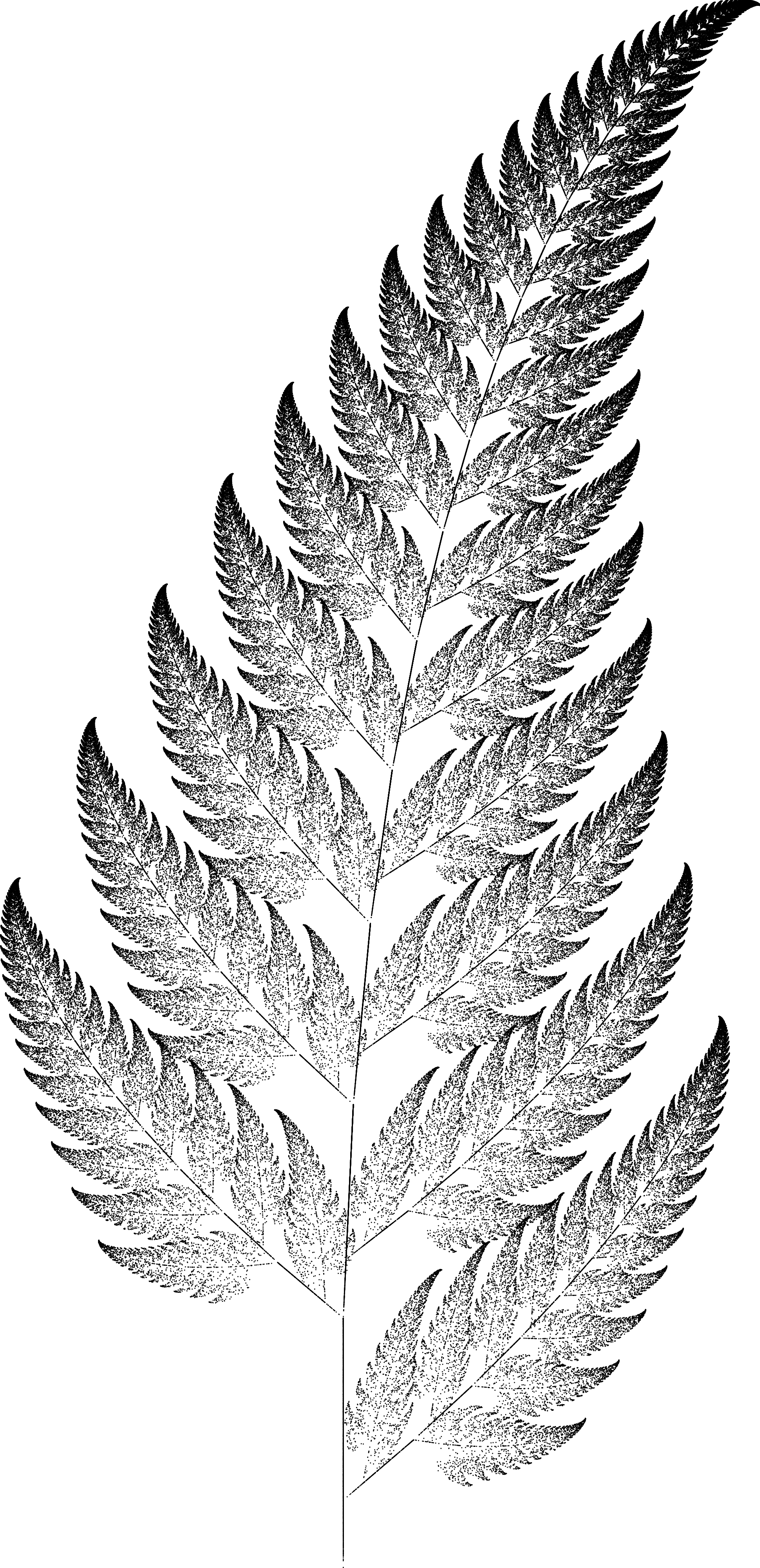
A famous example of a fractal based on iterated function systems is the Barnsley fern shown in Fig. 1.4. The fern consists of a stem that bends to the right and an infinite number of branches and leaves that are attached to the left and the right of the stem. Each branch is itself a scaled and rotated version of the Barnsley fern, as are the leaves of each branch: If you zoom into any part of the Barnsley fern, you find an endless number of smaller copies of the whole shape.

(image)

Figure 1.4 The Barnsley fern is a plant-like fractal that consists of countless smaller copies of itself (left). It is generated by four affine transformations, each of which corresponds to one part of the fractal (right).

The Barnsley fern is generated by an iterated function system that consists of four functions and four probabilities:

\begin{align*} f_0(\vec {p}) &= \begin{pmatrix} 0 & 0\\ 0 & 0.16 \end {pmatrix} \vec {p} + \begin{pmatrix} 0\\0 \end {pmatrix} & p_0=0.01 \\ f_1(\vec {p}) &= \begin{pmatrix} 0.85 & 0.04\\ -0.04 & 0.85 \end {pmatrix}\vec {p} + \begin{pmatrix} 0\\1.6 \end {pmatrix} & p_1=0.85 \\ f_2(\vec {p}) &= \begin{pmatrix} 0.2 & -0.26\\ 0.23 & 0.22 \end {pmatrix} \vec {p} + \begin{pmatrix} 0\\1.6 \end {pmatrix} & p_2=0.07 \\ f_3(\vec {p}) &= \begin{pmatrix} -0.15 & 0.28\\ 0.26 & 0.24 \end {pmatrix} \vec {p} + \begin{pmatrix} 0\\0.44 \end {pmatrix} & p_3=0.07 \end{align*} All four functions have the same form: They first multiply the vector \(\vec {p}\) by a \(2\times 2\) matrix and then translate the result by adding a vector. Functions of this form are called affine transformations, and they describe a wide range of geometric transformations such as rotation, scaling, shearing, and translation; see also Box 1.1.

Box 1.1: Linear and Affine Transformations Many important geometric transformations can be described mathematically using matrix operations. For example, scaling vectors by a constant factor \(\alpha \)

\[ \vec {p}\quad \mapsto \quad \alpha \vec {p} \]

can also be written as the matrix product

\[ \vec {p}\quad \mapsto \quad \begin {pmatrix} \alpha & 0 \\ 0 & \alpha \end {pmatrix} \vec {p}, \]

and similar matrix versions exist for other transformations such as rotation around the origin, shearing, and reflection. In general, a mapping that can be described by a matrix multiplication is called a linear transformation:

\begin{align*} \vec {p} \quad \mapsto \quad \vec {A}\vec {p} \qquad \text {or}\qquad \begin{pmatrix} x \\ y \end {pmatrix} \quad \mapsto \quad \begin{pmatrix} a & b\\ c & d \end {pmatrix} \begin{pmatrix} x \\ y \end {pmatrix} = \begin{pmatrix} ax + by\\ cx + dy \end {pmatrix}. \end{align*}

An important generalization of linear transformations are affine transformations, which first perform a matrix multiplication and then add a fixed vector \(\vec {t}\):

\begin{align*} \vec {p} \quad \mapsto \quad \vec {A}\vec {p} +\vec {t} \qquad \text {or}\qquad \begin{pmatrix} x \\ y \end {pmatrix} \quad \mapsto \quad \begin{pmatrix} a & b\\ c & d \end {pmatrix} \begin{pmatrix} x \\ y \end {pmatrix} + \begin{pmatrix} t_x \\ t_y \end {pmatrix} = \begin{pmatrix} ax + by + t_x\\ cx + dy + t_y \end {pmatrix}. \end{align*} Affine transformations let us rotate, scale, and shear as before, but they can also be used to move geometric objects in the plane. We will discuss affine transformations in more detail in Section 3.2.

The right part of Fig. 1.4 illustrates how these four affine transformations determine the shape and structure of the Barnsley fern. Imagine a rectangle that encloses the Barnsley fern and then transform this bounding box using each of the four transformations. The first transformation \(f_0\) flattens the box into a short vertical line that forms the stem of the fern; \(f_1\) moves a slightly scaled and rotated version of the bounding box to the end of the stem and generates the upper part of the fern; and the last two transformations \(f_2\) and \(f_3\) form the first leaf on the left and right of the fern, respectively. Notice that \(f_3\) also flips the coordinate system and introduces a slight shear, so the leaves on the right side of the fern bend to the left and are slightly skewed. Smaller details of the fern are obtained by applying multiple functions in sequence. For instance, applying \(f_2\) followed by \(f_0\) produces the stem of the left branch, and applying \(f_1\) followed by \(f_3\) the second branch on the right. Every part of the fractal corresponds to a particular combination of the four functions in its iterated function system; you can think of the four functions as the fractal’s geometric blueprint.

This geometric blueprint is filled with a random distribution of points using the chaos game. The probabilities \(p_1,\dots ,p_3\) control how the points are distributed over the different parts of the fractal: In the case of the Barnsley fern, the probabilities are \(0.01\), \(0.85\), \(0.07\), and \(0.07\), which means that approximately 1% of all points will be placed in the fern’s stem (or one of its many copies), 85% in its body, and 7% in the left and right leaves each. The four probabilities sum to 1, which reflects the fact that every point is allocated to one of the available transformations.

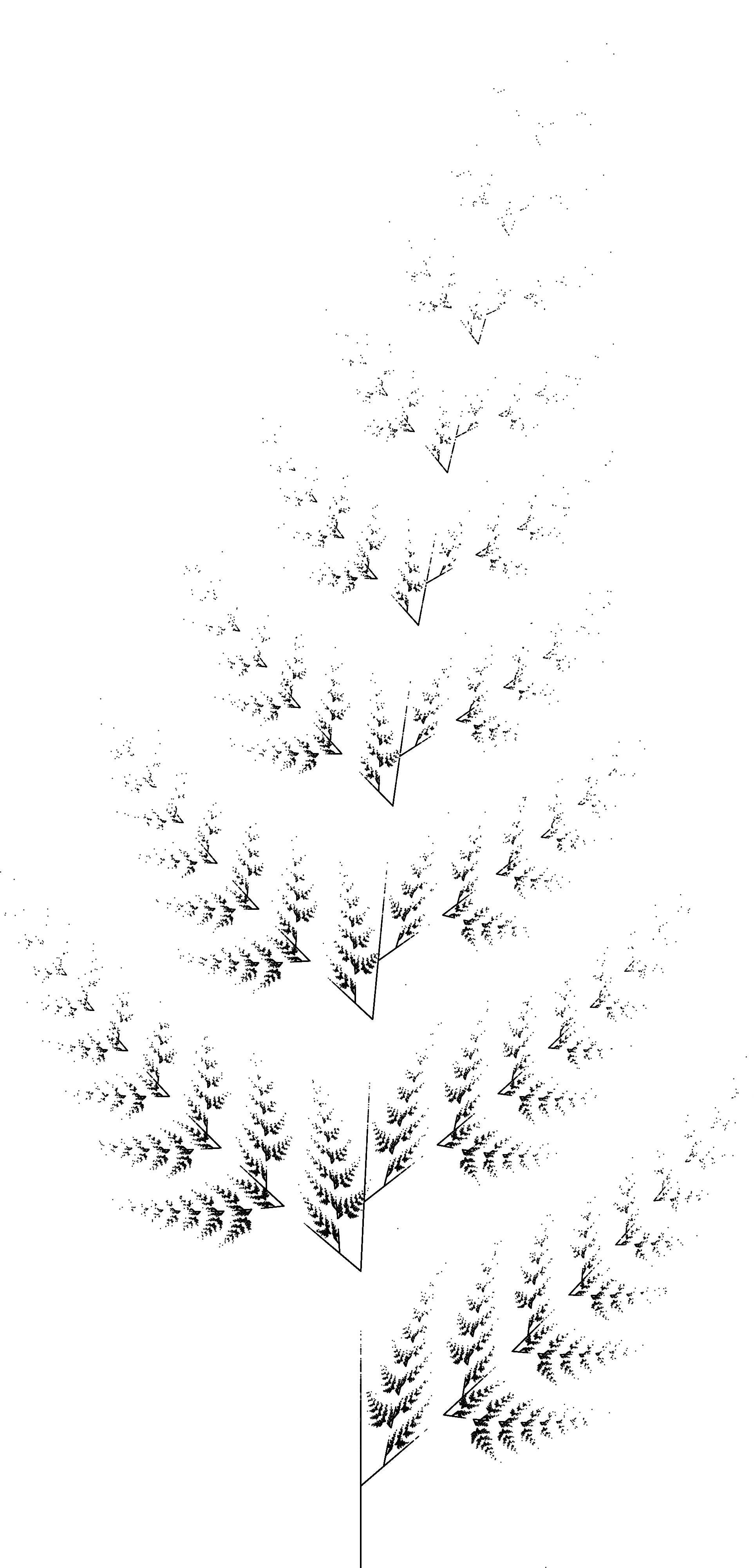
It is instructive to consider what happens if we choose other values for the probabilities. If we set all probabilities to \(1/4\), for instance, each part of the fractal receives the same number of points, and we obtain the rendering of the Barnsley fern shown in the left part of Fig. 1.5. With this choice of probabilities, most points end up in or close to the stem of the Barnsley fern and fewer points in its leaves. If, on the other hand, we set the four probabilities to 0.01, 0.94, 0.025, and 0.025, most points are allocated to the function \(f_1\), which increases the density of points in the tips of the branches, as illustrated in the right part of Fig. 1.5.

(image) (image)

Figure 1.5 The influence of IFS probabilities. The probabilities associated with an iterated function system determine the spatial distribution of points produced by the chaos game. Decreasing the probability of the stem places more points in the leaves (left) whereas increasing it emphasizes the stem but places fewer points in the leaves (right).

In practice, suitable values for the probabilities must usually be determined by trial and error, especially if the primary goal is to produce pleasing images. But it is possible to compute reasonable starting values so that more points end up in parts of the fractal that cover a large surface area; we will discuss one such an approach in Exercise 1.5.

Affine Iterated Function Systems

An affine transformation is a function that consists of a linear transformation — usually a combination of rotation, scaling, and shearing — followed by a translation. We usually write affine transformations in the following form:

\begin{equation} \label {eq:affine} \vec {p}\quad \mapsto \quad \begin{pmatrix} a & b\\ c & d \end {pmatrix}\vec {p} + \begin{pmatrix} t_x\\t_y \end {pmatrix}. \end{equation}

where \(\vec {p}\) is the point being transformed. The transform is completely defined by six numbers: the four coefficients \(a, b, c, d\) of the \(2\times 2\) matrix and the two coefficients \(t_x, t_y\) of the translation vector. To implement affine transformations, we define a record called Affine that stores these six numbers as floating-point numbers (Listing 1.5).

Listing 1.5ch1β€―/β€―Affine

// An affine transformation in 2D.
public record Affine(
        double a, double b,
        double c, double d,
        double tx, double ty) {
    // ...
}

If we set \(\vec {p}=\left (\begin {smallmatrix}x\\y\end {smallmatrix}\right )\) and expand the matrix product in Eq. (1.2), we obtain the coordinates \(x'\) and \(y'\) of the transformed point:

\begin{equation} \label {eq:affineapply} \begin{aligned} x' &= ax + by + t_x,\\ y' &= cx + dy + t_y. \end {aligned} \end{equation}

The transformPoint() method in Listing 1.6 uses this formula to apply an affine transformation to a given Point, producing a new Point. Since we will often work with lists of points, we also define a second method transformPoints() that transforms multiple points and returns the result as a new list. That’s all the functionality we need for now, although we will extend Affine with few additional methods in Chapter 3.

Listing 1.6ch1β€―/β€―Affine

// Transform a single point.
public Point transformPoint(Point p) {
    return new Point(a * p.x() + b * p.y() + tx,
            c * p.x() + d * p.y() + ty);
}

// Transform a list of points.
public List<Point> transformPoints(List<Point> points) {
    var result = new ArrayList<Point>(points.size());
    for (Point p : points)
        result.add(transformPoint(p));
    return result;
}

JDK: ArrayList, List
Affine
Point

We can now represent an affine iterated function system as an array of affine transformations of type Affine together with an array of probabilities of type double (Listing 1.7). The constructor of AffineIFS initializes transforms using the argument of the same name, but for probabilities it performs an additional normalization step to ensure that its entries sum to 1. Normalizing the probabilities ensures that exactly one of the affine transformations is chosen by the chaos game in each step. The second argument of AffineIFS() is therefore simply an array of frequencies that indicate how often each affine transformation is chosen relative to the others, which is then converted into a table of probabilities by dividing each entry by total, the sum of all frequencies.

Listing 1.7ch1β€―/β€―AffineIFS

// Representation of an affine iterated function system.
public class AffineIFS {
    public final Affine[] transforms;
    public final double[] probabilities;

    public AffineIFS(Affine[] transforms, double[] frequencies) {
        this.transforms = transforms;
        this.probabilities = new double[frequencies.length];
        double total = 0.0;
        for (double freq : frequencies)
            total += freq;
        for (int i = 0; i < frequencies.length; i++)
            this.probabilities[i] = frequencies[i] / total;
    }

    // ...
}

Affine

Listing 1.8 demonstrates how to construct an instance of AffineIFS that represents the Barnsley fern. In this case, the probabilities in the second array are already normalized.

Listing 1.8ch1β€―/β€―AffineIFS

public static AffineIFS BARNSLEY_FERN = new AffineIFS(
        new Affine[]{
                new Affine(0, 0, 0, 0.16, 0, 0),
                new Affine(0.85, 0.04, -0.04, 0.85, 0, 1.6),
                new Affine(0.2, -0.26, 0.23, 0.22, 0, 1.6),
                new Affine(-0.15, 0.28, 0.26, 0.24, 0, 0.44),
        },
        new double[]{0.01, 0.85, 0.07, 0.07}
);
The Extended Chaos Game

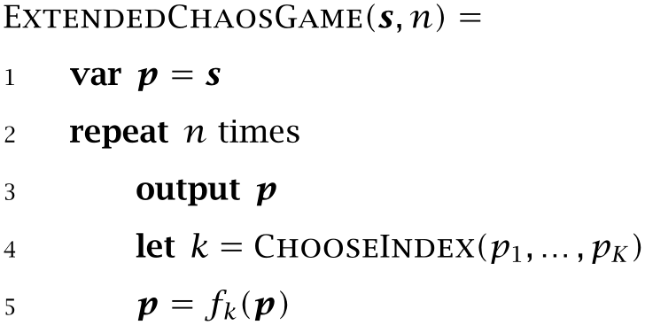
We can now turn to the problem of implementing the generalized version of the chaos game that lets us visualize the fractals described by affine iterated function systems. The formal description of this algorithm is shown in Algorithm 1.2. The main difference compared to the original chaos game in Algorithm 1.1 is that the algorithm now uses a fixed set of functions \(f_1,\dots , f_K\) and associated probabilities \(p_1,\dots ,p_K\) to move the current point in each step. In Line 4, we choose one of the functions by calling a function ChooseIndex, which returns an integer \(k\) between 1 and \(K\), and in Line 5, we move the current point \(\vec {p}\) to its new position by transforming it using the \(k\)th function \(f_k\).

Algorithm 1.2

Given a starting point \(\vec {s}\), produce a sequence of \(n\) points in the plane. The variables \(f_1,f_2,\dots f_K\) are affine transformations and \(p_1,p_2,\dots p_K\) the associated probabilities.

(image)

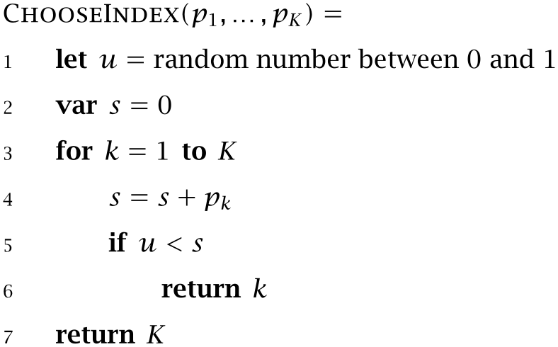
The job of the ChooseIndex function referenced in Algorithm 1.2 is to take a sequence of probabilities \(p_1,\dots ,p_K\) and generate a random index between 1 and \(K\) so that the integer \(k\) occurs with probability \(p_k\) (in other words, it returns the number 1 with probability \(p_1\), the number 2 with probability \(p_2\), and so on). How can we implement ChooseIndex?

One solution is to approach the problem geometrically. If the probabilities are normalized, we have \(p_1+\cdots +p_K=1\), which we can visualize by subdividing the interval \([0,1]\) into \(K\) sub-intervals of length \(p_1,p_2,\dots \):

The \(k\)th interval starts at \(p_1+\dots +p_{k-1}\) and ends at \(p_1+\dots +p_{k}\) and therefore has length \(p_k\). If we now pick a random real number \(u\) between 0 and 1, the probability that \(u\) lands in any particular sub-interval is obviously equal to the length of that interval, and the probability that it lands in the \(k\)th interval is \(p_k\). The index of the interval that contains \(u\) is therefore an integer between 1 and \(K\) with the desired probability distribution.

To find the interval that contains \(u\) we can simply try them one after another. If \(u<p_1\), the number lies in the leftmost interval with index \(k=1\); if \(u<p_0+p_1\), it lies in the second interval with index \(k=1\); otherwise, we continue in this manner until we find the first index \(k\) such that \(u<p_0+p_1+\dots +p_k\). The resulting algorithm is shown in Algorithm 1.3. The variable \(s\) accumulates the probabilities so it always contains the upper limit of the current interval, and the smallest index for which \(u < s\) is the desired random index.

Algorithm 1.3

Generate a random integer with a given distribution. The return value is an integer between 1 and \(K\), and the number \(k\) is returned with probability \(p_k\).

(image)

The generalized version of the chaos game can now be implemented as shown in Listing 1.9. The extendedChaosGame() method simulates the movement of the point start over the specified number of iterations and returns a list of visited points. In each iteration, the function appends the current position to points and then advances to the next point applying one of the affine transformations chosen at random. The chooseIndex() method implements the ChooseIndex algorithm: It uses the given random number generator to produce one floating point number between 0 and 1 and then searches for the interval that contains this number.

Listing 1.9ch1β€―/β€―AffineIFS

public List<Point> extendedChaosGame(
        Point start, int iterations, Random rng) {
    Point p = start;
    var points = new ArrayList<Point>(iterations);
    for (int i = 0; i < iterations; i++) {
        points.add(p);
        p = transforms[chooseIndex(rng)].transformPoint(p);
    }
    return points;
}

public int chooseIndex(Random rng) {
    double u = rng.nextDouble();
    double sum = 0.0;
    for (int i = 0; i < probabilities.length - 1; i++) {
        sum += probabilities[i];
        if (u < sum)
            return i;
    }
    return probabilities.length - 1;
}