As a slightly more complicated example of a recursive shape, consider the Pythagoras tree shown in Fig. 3.2. A Pythagoras tree consists of a square trunk from which two smaller Pythagoras trees branch off to form the boughs and ultimately the leaves of the tree.
Figure 3.2 The Pythagoras tree is constructed recursively: Every subtree consists of two smaller Pythagoras trees that are attached to a base square.
The basic building block of the Pythagoras tree is illustrated in Fig. 3.3. It consists of a base square and two attached smaller squares that form a right triangle with an inner angle \(\alpha \). The Pythagorean theorem \(a^2+b^2=c^2\), which relates the areas of the three squares, gives the tree its name. If we assume that the base square has side length 1, the long side of the triangle has length 1 and its two legs have length \(\cos \alpha \) and \(\sin \alpha \), respectively.
Figure 3.3 The main building block of a Pythagoras tree is a set of three squares that form a right triangle. If the base square has a side length of 1, the other two side lengths are \(\cos \alpha \) and \(\sin \alpha \).
We can compute the squares that make up the Pythagoras tree as follows. The idea is to find two sequences of geometric operations, let’s call them BranchL and BranchR, that transform the base square in Fig. 3.3 into the two squares that form
the left and right arm. If we transform the resulting two squares again using BranchL and BranchR, we obtain four additional squares, which are the root’s grandchildren in the Pythagoras tree. Every square in the tree can be computed by transforming the root square using a combination of transformation:
Starting at the root of the tree and moving toward the desired square, we apply BranchL every time we move to the left and BranchR every time we move to the right.
Here is how these two two transformations look. The left square can be obtained from the base square in three steps:
1. Scale the base square by a factor of \(\cos \alpha \) to make it the correct size.
2. Rotate the resulting square counterclockwise by the angle \(\alpha \) around its lower-left corner to give it the correct orientation.
3. Move it one unit upward so that its lower-left corner ends up at \((0,1)\).
The square that forms the right branch can be constructed similarly:
1. Move the base square one unit to the left so that its bottom-right corner coincides with the origin,
2. Scale by \(\sin \alpha \).
3. Rotate right by \(\pi /2-\alpha \).
4. Translate the resulting square to the upper-right corner of the base square.
Let’s introduce a few notations for specifying these types of geometric transformations. For a transformation that scales all coordinates by a factor \(a\) we write \(\text {Scale}(a)\); for the transformation that rotates points by an angle \(\phi \) we
write \(\text {Rotate}(\phi )\); and for the transformation that shifts points by an amount \(dx\) horizontally and by \(dy\) vertically we write \(\text {Translate}(dx, dy)\). If a sequence of geometric transformations are performed one after another, we write the individual
transformations in product form. This lets us we write the transformation \(\text {BranchL}\) that constructs the left branch of the Pythagoras tree by multiplying three individual transformations:
We follow the mathematical convention of writing a sequence of transformations from right to left, so the above definition states that BranchL first applies Scale(), then Rotate(), and finally Translate(). The transformation for the right branch of the Pythagoras tree can be written similarly as a sequence of
four geometric transformations:
Again, the right-hand side must be read from right to left: The right branch is constructed by translating, scaling, rotating, and then translating again.
Geometric Transformations
The three types of geometric transformations we just met — translation, rotation, and scaling — all belong to the class of affine transformations, which you may remember from our discussion of iterated function systems in Section 1.2. An affine transformation is a function that maps points to other points by multiplying them by
first a \(2\times 2\) matrix and then adding a vector to the result:
\(\seteqnumber{0}{3.}{2}\)
\begin{equation}
\vec {p}\quad \mapsto \quad \begin{pmatrix} a & b\\ c & d \end {pmatrix}\vec {p} + \begin{pmatrix} t_x\\t_y \end {pmatrix}.
\end{equation}
We already developed a class Affine for working with affine transformations in the previous chapter. The main constructor of Affine takes the six coefficients of the affine transformation as its arguments, so the general
transformation above is constructed as follows:
new Affine(a, b, c, d, tx, ty);
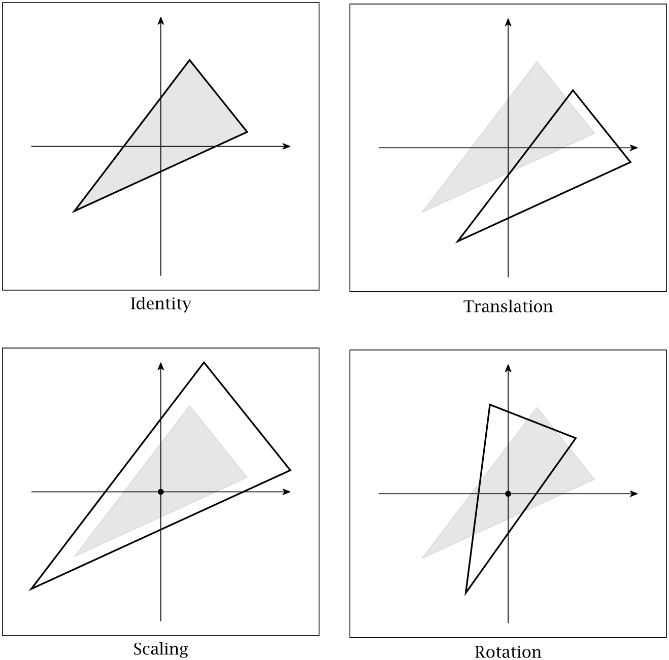
We will now discuss how to express the geometric transformations needed to construct the Pythagoras tree as affine transformations and how to extend Affine with methods for constructing them. The four affine transformations we
are interested in are illustrated in Fig. 3.4.
Figure 3.4 Elementary affine transformations. The identity transformation leaves the gray triangle unchanged, translation moves it by a fixed offset, scaling magnifies it relative to the origin, and rotation rotates it around the
origin.
Let’s start with a transformation we haven’t mentioned so far but that will turn out to be useful later on: The identity transformation, which maps every point to itself. It’s not hard to see that the only affine transformation that leaves every point unchanged has the following form:
This transformation first multiplies the point \(\vec {p}\) by the identity matrix \(\bigl (\begin {smallmatrix} 1 & 0\\ 0 & 1 \end {smallmatrix}\bigr )\) and then adds the zero vector \(\bigl (\begin {smallmatrix}0\\0\end {smallmatrix}\bigr )\).
The affine transformations for translation and scaling are simple variations of the identity transformation. A translation moves every point by a certain amount, say \(t_x\) units along the \(x\)-axis and \(t_y\) units along the \(y\)-axis. We can express this as an affine transformation by setting the matrix part to the identity matrix and the
translation vector to \(\bigl (\begin {smallmatrix}t_x\\t_y\end {smallmatrix}\bigr )\):
The scaling transformation multiplies all coordinates by a factor \(a\), which can be expressed as multiplying by a scaled version of the identity matrix followed by adding the zero vector:
\(\seteqnumber{0}{3.}{3}\)
\begin{equation*}
\begin{pmatrix} a & 0\\ 0 & a \end {pmatrix}\vec {p} + \begin{pmatrix} 0\\0 \end {pmatrix}\qquad \text {Scaling}
\end{equation*}
And finally, rotation by an angle \(\phi \) can be achieved by multiplying \(\vec {p}\) with a rotation matrix:
Listing 3.1 demonstrates how to create Affine objects that implement these four elementary transformations. The identity transformation can be defined as a static
variable since all its coefficients are constant. For the other three transformations, we define functions that take the required parameters as arguments and construct the corresponding Affine objects: translation() returns a transformation that moves every point by an offset dx horizontally and dy vertically; scaling() returns a transformation that scales both coordinates by a common factor, and rotation()
returns a transformation that rotates points by the given angle.
Listing 3.1ch1 / Affine
public static final Affine IDENTITY =
        new Affine(1, 0, 0, 1, 0, 0);

public static Affine translation(double dx, double dy) {
    return new Affine(1, 0, 0, 1, dx, dy);
}

public static Affine scaling(double factor) {
    return new Affine(factor, 0, 0, factor, 0, 0);
}

public static Affine rotation(double angle) {
    double cos = Math.cos(angle);
    double sin = Math.sin(angle);
    return new Affine(cos, -sin, sin, cos, 0, 0);
}
Using these elementary transformations as building blocks, we can perform many interesting geometric transformations by applying multiple Affine objects after another. For example, suppose we want to compute the left branch of
the Pythagoras tree using the BranchL transformation
This can be done by first computing the elementary transformations \(\text {Scale}(\cos \alpha )\), \(\text {Rotate}(\alpha )\), and \(\text {Translate}(0,1)\),
The corners of the transformed square are computed by applying these three transformations to the corners of the base square:
var baseShape = List.of(new Point(0, 0), new Point(1, 0),
        new Point(1, 1), new Point(0, 1));
var left = translateL.transformPoints(
        rotateL.transformPoints(scaleL.transformPoints(baseShape)));
To compute the next square along the left branch, we apply this sequence of transformations twice, for a total of six transformations. In general, the number of affine transformations we have to apply to compute a particular square in the Pythagoras tree increases with its distance from the root. Every time
we move left in the tree, we have to perform the three transformations of BranchL, and every time we move right, we have to perform the four transformations of BranchR.
It is possible to speed up these computations significantly by making use of an important property of affine transformations: they are composable, which means that the effect of multiple affine transformations applied one after the other is again an affine transformation. This is obvious in simple cases: For example, rotating first by \(40^\circ \) and then once more by \(30^\circ \) is equivalent
of rotating once by \(70^\circ \), and translating it first by a vector \(\vec {u}\) and then another vector \(\vec {v}\) is equivalent to translating once by \(\vec {u}+\vec {v}\).
In Exercise 3.3, we prove that this works for every pair of affine transformations: If \(A(\vec {p}) = \vec {A}\vec {p} + \vec {a}\) and \(B(\vec {p}) = \vec {B}\vec {p} + \vec {b}\), the function that corresponds to applying
\(A\) and \(B\) one after another
In other words, the matrix and vector parts of \(C\) are obtained by combining the parts of \(A\) and \(B\).
We will now use these identities to combine multiple Affine objects. First, we determine the coefficients of \(\vec {C}\) and \(\vec {c}\) by writing the transformations \(A\) and \(B\) in terms of their coefficients and then evaluating
the matrix products in Eq. (3.4). If we set
We can now define a method times() that multiplies this by another affine transformation t. The implementation shown in Listing 3.2 uses Eqs. (3.5) and (3.6) to compute
the coefficients of the new transformation.
Listing 3.2ch1 / Affine
public Affine times(Affine t) {
    return new Affine(a * t.a + b * t.c,
            a * t.b + b * t.d,
            c * t.a + d * t.c,
            c * t.b + d * t.d,
            a * t.tx + b * t.ty + tx,
            c * t.tx + d * t.ty + ty);
}
Because times() returns a new instance of Affine, calls to times() can be chained to apply multiple affine transformations in sequence. For example, we can construct the BranchL transformation for the left arm of the Pythagoras tree by starting with \(\text {Translate}(0,1)\) and then multiplying it successively by
\(\text {Rotate}(\alpha )\) and \(\text {Scale}(\cos \alpha )\):
Since sequences of affine transformations are so common in practice, we also define a second method compose() that takes multiple Affine objects and
collapses them into a single transformation (Listing 3.3). Similar to the way we just constructed branchL in the previous example, the function combines the transformations by accumulating their product using times(). Notice that this implementation of compose() also works correctly if the argument
transforms is either empty or contains just a single element: Since result is initialized to the identity transformation, the composition of zero transformations returns IDENTITY, and the composition of one transformation returns that
transformation itself.
Listing 3.3ch1 / Affine
public static Affine compose(Affine... transforms) {
    Affine result = IDENTITY;
    for (Affine t : transforms)
        result = result.times(t);
    return result;
}
Using compose() we can construct the transformation that computes the left branch using a notation that is even closer to the mathematical definition in Eq. (3.1):
Exercise 3.3. Show that the combination of two affine transformations \(A(\vec {p}) = \vec {A}\vec {p} + \vec {a}\) and \(B(\vec {p}) = \vec {B}\vec {p} + \vec
{b}\) is another affine transformation \(C\) and derive Eq. (3.4).