11 Big Integers
\(\newcommand{\footnotename}{footnote}\)
\(\def \LWRfootnote {1}\)
\(\newcommand {\footnote }[2][\LWRfootnote ]{{}^{\mathrm {#1}}}\)
\(\newcommand {\footnotemark }[1][\LWRfootnote ]{{}^{\mathrm {#1}}}\)
\(\let \LWRorighspace \hspace \)
\(\renewcommand {\hspace }{\ifstar \LWRorighspace \LWRorighspace }\)
\(\newcommand {\TextOrMath }[2]{#2}\)
\(\newcommand {\mathnormal }[1]{{#1}}\)
\(\newcommand \ensuremath [1]{#1}\)
\(\newcommand {\LWRframebox }[2][]{\fbox {#2}} \newcommand {\framebox }[1][]{\LWRframebox } \)
\(\newcommand {\setlength }[2]{}\)
\(\newcommand {\addtolength }[2]{}\)
\(\newcommand {\setcounter }[2]{}\)
\(\newcommand {\addtocounter }[2]{}\)
\(\newcommand {\arabic }[1]{}\)
\(\newcommand {\number }[1]{}\)
\(\newcommand {\noalign }[1]{\text {#1}\notag \\}\)
\(\newcommand {\cline }[1]{}\)
\(\newcommand {\directlua }[1]{\text {(directlua)}}\)
\(\newcommand {\luatexdirectlua }[1]{\text {(directlua)}}\)
\(\newcommand {\protect }{}\)
\(\def \LWRabsorbnumber #1 {}\)
\(\def \LWRabsorbquotenumber "#1 {}\)
\(\newcommand {\LWRabsorboption }[1][]{}\)
\(\newcommand {\LWRabsorbtwooptions }[1][]{\LWRabsorboption }\)
\(\def \mathchar {\ifnextchar "\LWRabsorbquotenumber \LWRabsorbnumber }\)
\(\def \mathcode #1={\mathchar }\)
\(\let \delcode \mathcode \)
\(\let \delimiter \mathchar \)
\(\def \oe {\unicode {x0153}}\)
\(\def \OE {\unicode {x0152}}\)
\(\def \ae {\unicode {x00E6}}\)
\(\def \AE {\unicode {x00C6}}\)
\(\def \aa {\unicode {x00E5}}\)
\(\def \AA {\unicode {x00C5}}\)
\(\def \o {\unicode {x00F8}}\)
\(\def \O {\unicode {x00D8}}\)
\(\def \l {\unicode {x0142}}\)
\(\def \L {\unicode {x0141}}\)
\(\def \ss {\unicode {x00DF}}\)
\(\def \SS {\unicode {x1E9E}}\)
\(\def \dag {\unicode {x2020}}\)
\(\def \ddag {\unicode {x2021}}\)
\(\def \P {\unicode {x00B6}}\)
\(\def \copyright {\unicode {x00A9}}\)
\(\def \pounds {\unicode {x00A3}}\)
\(\let \LWRref \ref \)
\(\renewcommand {\ref }{\ifstar \LWRref \LWRref }\)
\( \newcommand {\multicolumn }[3]{#3}\)
\(\require {textcomp}\)
\(\newcommand {\intertext }[1]{\text {#1}\notag \\}\)
\(\let \Hat \hat \)
\(\let \Check \check \)
\(\let \Tilde \tilde \)
\(\let \Acute \acute \)
\(\let \Grave \grave \)
\(\let \Dot \dot \)
\(\let \Ddot \ddot \)
\(\let \Breve \breve \)
\(\let \Bar \bar \)
\(\let \Vec \vec \)
\(\renewcommand {\vec }{\boldsymbol }\)
\(\newcommand {\Edge }{\ensuremath {\,\textemdash \,}}\)
\(\newcommand \Const [1]{\text {\textsf {#1}}}\)
\(\DeclareMathOperator {\lerp }{lerp}\)
\(\DeclareMathOperator {\bitlen }{bitlen}\)
\(\DeclareMathOperator {\sign }{sign}\)
\(\newcommand {\I }{\mathrm {i}}\)
\(\newcommand \AND {\mathbin {\&}}\)
\(\newcommand \OR {\mathbin {|}}\)
\(\newcommand \XOR {\mathbin {{}^{\wedge }}}\)
\(\newcommand \shl {\ll }\)
\(\newcommand \shr {\ggg }\)
\(\newcommand \asr {\gg }\)
\(\newcommand \NOT {\ensuremath {\mathord {\sim }}}\)
\(\newcommand {\isep }{\mathrel {{.}\,{.}}}\)
\(\newcommand {\Id }[1]{\mathit {#1}}\)
\(\newcommand {\const }[1]{\mathsf {#1}}\)
\(\newcommand {\algorithmname }[1]{\text {\textsc {#1}}}\)
\(\newcommand {\bits }[1]{\text {#1}}\)
\(\newcommand {\hexa }[1]{\mathtt {0x#1}}\)
\(\newcommand {\num }[1]{#1}\)
\(\newcommand {\qed }{\quad \square }\)
\(\newcommand {\idiv }[2]{\lfloor #1/#2\rfloor }\)
\(\newcommand \attribdot {\ensuremath {\mkern 1.5mu.\mkern 1.5mu}}\)
\(\newcommand \attribxr [2]{#1\attribdot \text {#2}}\)
\(\newcommand \attribir [2]{\Id {#1}\attribdot \text {#2}}\)
\(\newcommand \attribii [2]{\Id {#1}\attribdot \Id {#2}}\)
\(\newcommand \textsc [1]{#1}\)
\(\require {colortbl}\)
\(\let \LWRorigcolumncolor \columncolor \)
\(\renewcommand {\columncolor }[2][named]{\LWRorigcolumncolor [#1]{#2}\LWRabsorbtwooptions }\)
\(\let \LWRorigrowcolor \rowcolor \)
\(\renewcommand {\rowcolor }[2][named]{\LWRorigrowcolor [#1]{#2}\LWRabsorbtwooptions }\)
\(\let \LWRorigcellcolor \cellcolor \)
\(\renewcommand {\cellcolor }[2][named]{\LWRorigcellcolor [#1]{#2}\LWRabsorbtwooptions }\)
\(\newcommand {\tcbset }[1]{}\)
\(\newcommand {\tcbsetforeverylayer }[1]{}\)
\(\newcommand {\tcbox }[2][]{\boxed {\text {#2}}}\)
\(\newcommand {\tcboxfit }[2][]{\boxed {#2}}\)
\(\newcommand {\tcblower }{}\)
\(\newcommand {\tcbline }{}\)
\(\newcommand {\tcbtitle }{}\)
\(\newcommand {\tcbsubtitle [2][]{\mathrm {#2}}}\)
\(\newcommand {\tcboxmath }[2][]{\boxed {#2}}\)
\(\newcommand {\tcbhighmath }[2][]{\boxed {#2}}\)
\(\newcommand {\toprule }[1][]{\hline }\)
\(\let \midrule \toprule \)
\(\let \bottomrule \toprule \)
\(\def \LWRbooktabscmidruleparen (#1)#2{}\)
\(\newcommand {\LWRbooktabscmidrulenoparen }[1]{}\)
\(\newcommand {\cmidrule }[1][]{\ifnextchar (\LWRbooktabscmidruleparen \LWRbooktabscmidrulenoparen }\)
\(\newcommand {\morecmidrules }{}\)
\(\newcommand {\specialrule }[3]{\hline }\)
\(\newcommand {\addlinespace }[1][]{}\)
\(\newcommand {\LWRsubmultirow }[2][]{#2}\)
\(\newcommand {\LWRmultirow }[2][]{\LWRsubmultirow }\)
\(\newcommand {\multirow }[2][]{\LWRmultirow }\)
\(\newcommand {\mrowcell }{}\)
\(\newcommand {\mcolrowcell }{}\)
\(\newcommand {\STneed }[1]{}\)
\(\newcommand {\LWRldelimtwo }[1][]{\text {#1}~\LWRbigdelim }\)
\(\newcommand {\LWRldelimone }[2][]{\LWRldelimtwo }\)
\(\def \ldelim #1#2{\def \LWRbigdelim {#1}\LWRldelimone }\)
\(\newcommand {\LWRrdelimtwo }[1][]{\LWRbigdelim ~\text {#1}}\)
\(\newcommand {\LWRrdelimone }[2][]{\LWRrdelimtwo }\)
\(\def \rdelim #1#2{\def \LWRbigdelim {#1}\LWRrdelimone }\)
\(\let \symnormal \mathit \)
\(\let \symliteral \mathrm \)
\(\let \symbb \mathbb \)
\(\let \symbbit \mathbb \)
\(\let \symcal \mathcal \)
\(\let \symscr \mathscr \)
\(\let \symfrak \mathfrak \)
\(\let \symsfup \mathsf \)
\(\let \symsfit \mathit \)
\(\let \symbfsf \mathbf \)
\(\let \symbfup \mathbf \)
\(\newcommand {\symbfit }[1]{\boldsymbol {#1}}\)
\(\let \symbfcal \mathcal \)
\(\let \symbfscr \mathscr \)
\(\let \symbffrak \mathfrak \)
\(\let \symbfsfup \mathbf \)
\(\newcommand {\symbfsfit }[1]{\boldsymbol {#1}}\)
\(\let \symup \mathrm \)
\(\let \symbf \mathbf \)
\(\let \symit \mathit \)
\(\let \symsf \symsfit \)
\(\let \symtt \mathtt \)
\(\let \symbffrac \mathbffrac \)
\(\newcommand {\mathfence }[1]{\mathord {#1}}\)
\(\newcommand {\mathover }[1]{#1}\)
\(\newcommand {\mathunder }[1]{#1}\)
\(\newcommand {\mathaccent }[1]{#1}\)
\(\newcommand {\mathbotaccent }[1]{#1}\)
\(\newcommand {\mathalpha }[1]{\mathord {#1}}\)
\(\def\Alpha{\unicode{x1D6E2}}\)
\(\def\Beta{\unicode{x1D6E3}}\)
\(\def\Gamma{\unicode{x1D6E4}}\)
\(\def\Digamma{\mathit{\unicode{x03DC}}}\)
\(\def\Delta{\unicode{x1D6E5}}\)
\(\def\Epsilon{\unicode{x1D6E6}}\)
\(\def\Zeta{\unicode{x1D6E7}}\)
\(\def\Eta{\unicode{x1D6E8}}\)
\(\def\Theta{\unicode{x1D6E9}}\)
\(\def\Vartheta{\unicode{x1D6F3}}\)
\(\def\Iota{\unicode{x1D6EA}}\)
\(\def\Kappa{\unicode{x1D6EB}}\)
\(\def\Lambda{\unicode{x1D6EC}}\)
\(\def\Mu{\unicode{x1D6ED}}\)
\(\def\Nu{\unicode{x1D6EE}}\)
\(\def\Xi{\unicode{x1D6EF}}\)
\(\def\Omicron{\unicode{x1D6F0}}\)
\(\def\Pi{\unicode{x1D6F1}}\)
\(\def\Rho{\unicode{x1D6F2}}\)
\(\def\Sigma{\unicode{x1D6F4}}\)
\(\def\Tau{\unicode{x1D6F5}}\)
\(\def\Upsilon{\unicode{x1D6F6}}\)
\(\def\Phi{\unicode{x1D6F7}}\)
\(\def\Chi{\unicode{x1D6F8}}\)
\(\def\Psi{\unicode{x1D6F9}}\)
\(\def\Omega{\unicode{x1D6FA}}\)
\(\def\alpha{\unicode{x1D6FC}}\)
\(\def\beta{\unicode{x1D6FD}}\)
\(\def\varbeta{\unicode{x03D0}}\)
\(\def\gamma{\unicode{x1D6FE}}\)
\(\def\digamma{\mathit{\unicode{x03DD}}}\)
\(\def\delta{\unicode{x1D6FF}}\)
\(\def\epsilon{\unicode{x1D716}}\)
\(\def\varepsilon{\unicode{x1D700}}\)
\(\def\zeta{\unicode{x1D701}}\)
\(\def\eta{\unicode{x1D702}}\)
\(\def\theta{\unicode{x1D703}}\)
\(\def\vartheta{\unicode{x1D717}}\)
\(\def\iota{\unicode{x1D704}}\)
\(\def\kappa{\unicode{x1D705}}\)
\(\def\varkappa{\unicode{x1D718}}\)
\(\def\lambda{\unicode{x1D706}}\)
\(\def\mu{\unicode{x1D707}}\)
\(\def\nu{\unicode{x1D708}}\)
\(\def\xi{\unicode{x1D709}}\)
\(\def\omicron{\unicode{x1D70A}}\)
\(\def\pi{\unicode{x1D70B}}\)
\(\def\varpi{\unicode{x1D71B}}\)
\(\def\rho{\unicode{x1D70C}}\)
\(\def\varrho{\unicode{x1D71A}}\)
\(\def\sigma{\unicode{x1D70E}}\)
\(\def\varsigma{\unicode{x1D70D}}\)
\(\def\tau{\unicode{x1D70F}}\)
\(\def\upsilon{\unicode{x1D710}}\)
\(\def\phi{\unicode{x1D719}}\)
\(\def\varphi{\unicode{x1D711}}\)
\(\def\chi{\unicode{x1D712}}\)
\(\def\psi{\unicode{x1D713}}\)
\(\def\omega{\unicode{x1D714}}\)
\(\def\upAlpha{\unicode{x0391}}\)
\(\def\upBeta{\unicode{x0392}}\)
\(\def\upGamma{\unicode{x0393}}\)
\(\def\upDigamma{\unicode{x03DC}}\)
\(\def\upDelta{\unicode{x0394}}\)
\(\def\upEpsilon{\unicode{x0395}}\)
\(\def\upZeta{\unicode{x0396}}\)
\(\def\upEta{\unicode{x0397}}\)
\(\def\upTheta{\unicode{x0398}}\)
\(\def\upVartheta{\unicode{x03F4}}\)
\(\def\upIota{\unicode{x0399}}\)
\(\def\upKappa{\unicode{x039A}}\)
\(\def\upLambda{\unicode{x039B}}\)
\(\def\upMu{\unicode{x039C}}\)
\(\def\upNu{\unicode{x039D}}\)
\(\def\upXi{\unicode{x039E}}\)
\(\def\upOmicron{\unicode{x039F}}\)
\(\def\upPi{\unicode{x03A0}}\)
\(\def\upVarpi{\unicode{x03D6}}\)
\(\def\upRho{\unicode{x03A1}}\)
\(\def\upSigma{\unicode{x03A3}}\)
\(\def\upTau{\unicode{x03A4}}\)
\(\def\upUpsilon{\unicode{x03A5}}\)
\(\def\upPhi{\unicode{x03A6}}\)
\(\def\upChi{\unicode{x03A7}}\)
\(\def\upPsi{\unicode{x03A8}}\)
\(\def\upOmega{\unicode{x03A9}}\)
\(\def\itAlpha{\unicode{x1D6E2}}\)
\(\def\itBeta{\unicode{x1D6E3}}\)
\(\def\itGamma{\unicode{x1D6E4}}\)
\(\def\itDigamma{\mathit{\unicode{x03DC}}}\)
\(\def\itDelta{\unicode{x1D6E5}}\)
\(\def\itEpsilon{\unicode{x1D6E6}}\)
\(\def\itZeta{\unicode{x1D6E7}}\)
\(\def\itEta{\unicode{x1D6E8}}\)
\(\def\itTheta{\unicode{x1D6E9}}\)
\(\def\itVartheta{\unicode{x1D6F3}}\)
\(\def\itIota{\unicode{x1D6EA}}\)
\(\def\itKappa{\unicode{x1D6EB}}\)
\(\def\itLambda{\unicode{x1D6EC}}\)
\(\def\itMu{\unicode{x1D6ED}}\)
\(\def\itNu{\unicode{x1D6EE}}\)
\(\def\itXi{\unicode{x1D6EF}}\)
\(\def\itOmicron{\unicode{x1D6F0}}\)
\(\def\itPi{\unicode{x1D6F1}}\)
\(\def\itRho{\unicode{x1D6F2}}\)
\(\def\itSigma{\unicode{x1D6F4}}\)
\(\def\itTau{\unicode{x1D6F5}}\)
\(\def\itUpsilon{\unicode{x1D6F6}}\)
\(\def\itPhi{\unicode{x1D6F7}}\)
\(\def\itChi{\unicode{x1D6F8}}\)
\(\def\itPsi{\unicode{x1D6F9}}\)
\(\def\itOmega{\unicode{x1D6FA}}\)
\(\def\upalpha{\unicode{x03B1}}\)
\(\def\upbeta{\unicode{x03B2}}\)
\(\def\upvarbeta{\unicode{x03D0}}\)
\(\def\upgamma{\unicode{x03B3}}\)
\(\def\updigamma{\unicode{x03DD}}\)
\(\def\updelta{\unicode{x03B4}}\)
\(\def\upepsilon{\unicode{x03F5}}\)
\(\def\upvarepsilon{\unicode{x03B5}}\)
\(\def\upzeta{\unicode{x03B6}}\)
\(\def\upeta{\unicode{x03B7}}\)
\(\def\uptheta{\unicode{x03B8}}\)
\(\def\upvartheta{\unicode{x03D1}}\)
\(\def\upiota{\unicode{x03B9}}\)
\(\def\upkappa{\unicode{x03BA}}\)
\(\def\upvarkappa{\unicode{x03F0}}\)
\(\def\uplambda{\unicode{x03BB}}\)
\(\def\upmu{\unicode{x03BC}}\)
\(\def\upnu{\unicode{x03BD}}\)
\(\def\upxi{\unicode{x03BE}}\)
\(\def\upomicron{\unicode{x03BF}}\)
\(\def\uppi{\unicode{x03C0}}\)
\(\def\upvarpi{\unicode{x03D6}}\)
\(\def\uprho{\unicode{x03C1}}\)
\(\def\upvarrho{\unicode{x03F1}}\)
\(\def\upsigma{\unicode{x03C3}}\)
\(\def\upvarsigma{\unicode{x03C2}}\)
\(\def\uptau{\unicode{x03C4}}\)
\(\def\upupsilon{\unicode{x03C5}}\)
\(\def\upphi{\unicode{x03D5}}\)
\(\def\upvarphi{\unicode{x03C6}}\)
\(\def\upchi{\unicode{x03C7}}\)
\(\def\uppsi{\unicode{x03C8}}\)
\(\def\upomega{\unicode{x03C9}}\)
\(\def\italpha{\unicode{x1D6FC}}\)
\(\def\itbeta{\unicode{x1D6FD}}\)
\(\def\itvarbeta{\unicode{x03D0}}\)
\(\def\itgamma{\unicode{x1D6FE}}\)
\(\def\itdigamma{\mathit{\unicode{x03DD}}}\)
\(\def\itdelta{\unicode{x1D6FF}}\)
\(\def\itepsilon{\unicode{x1D716}}\)
\(\def\itvarepsilon{\unicode{x1D700}}\)
\(\def\itzeta{\unicode{x1D701}}\)
\(\def\iteta{\unicode{x1D702}}\)
\(\def\ittheta{\unicode{x1D703}}\)
\(\def\itvartheta{\unicode{x1D717}}\)
\(\def\itiota{\unicode{x1D704}}\)
\(\def\itkappa{\unicode{x1D705}}\)
\(\def\itvarkappa{\unicode{x1D718}}\)
\(\def\itlambda{\unicode{x1D706}}\)
\(\def\itmu{\unicode{x1D707}}\)
\(\def\itnu{\unicode{x1D708}}\)
\(\def\itxi{\unicode{x1D709}}\)
\(\def\itomicron{\unicode{x1D70A}}\)
\(\def\itpi{\unicode{x1D70B}}\)
\(\def\itvarpi{\unicode{x1D71B}}\)
\(\def\itrho{\unicode{x1D70C}}\)
\(\def\itvarrho{\unicode{x1D71A}}\)
\(\def\itsigma{\unicode{x1D70E}}\)
\(\def\itvarsigma{\unicode{x1D70D}}\)
\(\def\ittau{\unicode{x1D70F}}\)
\(\def\itupsilon{\unicode{x1D710}}\)
\(\def\itphi{\unicode{x1D719}}\)
\(\def\itvarphi{\unicode{x1D711}}\)
\(\def\itchi{\unicode{x1D712}}\)
\(\def\itpsi{\unicode{x1D713}}\)
\(\def\itomega{\unicode{x1D714}}\)
\(\let \lparen (\)
\(\let \rparen )\)
\(\newcommand {\cuberoot }[1]{\,{}^3\!\!\sqrt {#1}}\,\)
\(\newcommand {\fourthroot }[1]{\,{}^4\!\!\sqrt {#1}}\,\)
\(\newcommand {\longdivision }[1]{\mathord {\unicode {x027CC}#1}}\)
\(\newcommand {\mathcomma }{,}\)
\(\newcommand {\mathcolon }{:}\)
\(\newcommand {\mathsemicolon }{;}\)
\(\newcommand {\overbracket }[1]{\mathinner {\overline {\ulcorner {#1}\urcorner }}}\)
\(\newcommand {\underbracket }[1]{\mathinner {\underline {\llcorner {#1}\lrcorner }}}\)
\(\newcommand {\overbar }[1]{\mathord {#1\unicode {x00305}}}\)
\(\newcommand {\ovhook }[1]{\mathord {#1\unicode {x00309}}}\)
\(\newcommand {\ocirc }[1]{\mathord {#1\unicode {x0030A}}}\)
\(\newcommand {\candra }[1]{\mathord {#1\unicode {x00310}}}\)
\(\newcommand {\oturnedcomma }[1]{\mathord {#1\unicode {x00312}}}\)
\(\newcommand {\ocommatopright }[1]{\mathord {#1\unicode {x00315}}}\)
\(\newcommand {\droang }[1]{\mathord {#1\unicode {x0031A}}}\)
\(\newcommand {\leftharpoonaccent }[1]{\mathord {#1\unicode {x020D0}}}\)
\(\newcommand {\rightharpoonaccent }[1]{\mathord {#1\unicode {x020D1}}}\)
\(\newcommand {\vertoverlay }[1]{\mathord {#1\unicode {x020D2}}}\)
\(\newcommand {\leftarrowaccent }[1]{\mathord {#1\unicode {x020D0}}}\)
\(\newcommand {\annuity }[1]{\mathord {#1\unicode {x020E7}}}\)
\(\newcommand {\widebridgeabove }[1]{\mathord {#1\unicode {x020E9}}}\)
\(\newcommand {\asteraccent }[1]{\mathord {#1\unicode {x020F0}}}\)
\(\newcommand {\threeunderdot }[1]{\mathord {#1\unicode {x020E8}}}\)
\(\newcommand {\Bbbsum }{\mathop {\unicode {x2140}}\limits }\)
\(\newcommand {\oiint }{\mathop {\unicode {x222F}}\limits }\)
\(\newcommand {\oiiint }{\mathop {\unicode {x2230}}\limits }\)
\(\newcommand {\intclockwise }{\mathop {\unicode {x2231}}\limits }\)
\(\newcommand {\ointclockwise }{\mathop {\unicode {x2232}}\limits }\)
\(\newcommand {\ointctrclockwise }{\mathop {\unicode {x2233}}\limits }\)
\(\newcommand {\varointclockwise }{\mathop {\unicode {x2232}}\limits }\)
\(\newcommand {\leftouterjoin }{\mathop {\unicode {x27D5}}\limits }\)
\(\newcommand {\rightouterjoin }{\mathop {\unicode {x27D6}}\limits }\)
\(\newcommand {\fullouterjoin }{\mathop {\unicode {x27D7}}\limits }\)
\(\newcommand {\bigbot }{\mathop {\unicode {x27D8}}\limits }\)
\(\newcommand {\bigtop }{\mathop {\unicode {x27D9}}\limits }\)
\(\newcommand {\xsol }{\mathop {\unicode {x29F8}}\limits }\)
\(\newcommand {\xbsol }{\mathop {\unicode {x29F9}}\limits }\)
\(\newcommand {\bigcupdot }{\mathop {\unicode {x2A03}}\limits }\)
\(\newcommand {\bigsqcap }{\mathop {\unicode {x2A05}}\limits }\)
\(\newcommand {\conjquant }{\mathop {\unicode {x2A07}}\limits }\)
\(\newcommand {\disjquant }{\mathop {\unicode {x2A08}}\limits }\)
\(\newcommand {\bigtimes }{\mathop {\unicode {x2A09}}\limits }\)
\(\newcommand {\modtwosum }{\mathop {\unicode {x2A0A}}\limits }\)
\(\newcommand {\sumint }{\mathop {\unicode {x2A0B}}\limits }\)
\(\newcommand {\intbar }{\mathop {\unicode {x2A0D}}\limits }\)
\(\newcommand {\intBar }{\mathop {\unicode {x2A0E}}\limits }\)
\(\newcommand {\fint }{\mathop {\unicode {x2A0F}}\limits }\)
\(\newcommand {\cirfnint }{\mathop {\unicode {x2A10}}\limits }\)
\(\newcommand {\awint }{\mathop {\unicode {x2A11}}\limits }\)
\(\newcommand {\rppolint }{\mathop {\unicode {x2A12}}\limits }\)
\(\newcommand {\scpolint }{\mathop {\unicode {x2A13}}\limits }\)
\(\newcommand {\npolint }{\mathop {\unicode {x2A14}}\limits }\)
\(\newcommand {\pointint }{\mathop {\unicode {x2A15}}\limits }\)
\(\newcommand {\sqint }{\mathop {\unicode {x2A16}}\limits }\)
\(\newcommand {\intlarhk }{\mathop {\unicode {x2A17}}\limits }\)
\(\newcommand {\intx }{\mathop {\unicode {x2A18}}\limits }\)
\(\newcommand {\intcap }{\mathop {\unicode {x2A19}}\limits }\)
\(\newcommand {\intcup }{\mathop {\unicode {x2A1A}}\limits }\)
\(\newcommand {\upint }{\mathop {\unicode {x2A1B}}\limits }\)
\(\newcommand {\lowint }{\mathop {\unicode {x2A1C}}\limits }\)
\(\newcommand {\bigtriangleleft }{\mathop {\unicode {x2A1E}}\limits }\)
\(\newcommand {\zcmp }{\mathop {\unicode {x2A1F}}\limits }\)
\(\newcommand {\zpipe }{\mathop {\unicode {x2A20}}\limits }\)
\(\newcommand {\zproject }{\mathop {\unicode {x2A21}}\limits }\)
\(\newcommand {\biginterleave }{\mathop {\unicode {x2AFC}}\limits }\)
\(\newcommand {\bigtalloblong }{\mathop {\unicode {x2AFF}}\limits }\)
\(\newcommand {\arabicmaj }{\mathop {\unicode {x1EEF0}}\limits }\)
\(\newcommand {\arabichad }{\mathop {\unicode {x1EEF1}}\limits }\)
11.4 Multiplication
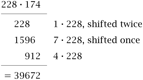
To find the algorithm for multiplication, we again start with the familiar pen-and-paper method for multiplying decimal numbers. Assume we want to compute \(228\cdot 174\). To do this, we first replace one of the arguments with its decimal expansion, which in this case gives us
\(\seteqnumber{0}{11.}{3}\)
\begin{equation*}
228\cdot (100 + 70 + 4) = 228\cdot 100 + 228\cdot 70 + 228\cdot 4.
\end{equation*}
Every term on the right-hand side multiplies \(228\) by a number of the form \(10^ky_k\), where \(y_k\) is the \(k\)th digit of \(y=174\). Since multiplication by a power of 10 is equivalent to shifting decimal digits to the left, we can also visualize this process as follows:
The result on the final line is obtained by adding the three intermediate results above it.
Generalizing this idea base-\(B\) integers is straightforward. Again, we first rewrite the product of \(x\) and \(y\) by expanding the multiplier, which reduces the problem of computing \(x\cdot y\) to the simpler problems of multiplying \(x\) by the digits \(y_k\) and then shifting and
adding the resulting terms:
\(\seteqnumber{0}{11.}{3}\)
\begin{equation}
\label {eq:multiply} xy=x\cdot \sum _{k=0}^ny_kB^k = \sum _{k=0}^n x y_kB^k.
\end{equation}
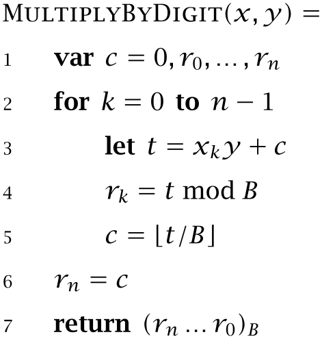
Each product \(x\cdot y_k\) can be computed by multiplying the digits of \(x\) by \(y_k\), starting with the least significant digit and propagating overflows to more significant digits. The resulting algorithm is shown in Algorithm 11.3; except for the computation of \(t\) on line 3, it is identical to the Add
algorithm we discussed in the previous section (Algorithm 11.1). With a small modification, MultiplyByDigit can also be used to multiply a
number \(x\) by a factor of the form \(y B^{m}\). The only effect of the additional factor \(B^m\) is to shift the digits of the result by \(m\) places, so we simply multiply by \(y\) as before and store each digit in \(r_{k+m}\) instead of \(r_k\).
Multiply a big integer \(x=(x_{n-1}\ldots x_0)_B\) by a single digit \(y\). The result is a \(n+1\)-digit integer \((r_n\ldots r_0)_B\).
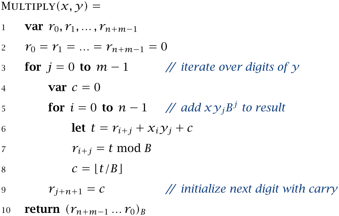
To complete the implementation of Eq. (11.4) and obtain the full multiplication algorithm for big integers, we need to wrap MultiplyByDigit in an outer loop that iterates over the digits \(y_k\) of the multiplicator and accumulates all intermediate products \(xy_kB^k\). The resulting algorithm is shown in Algorithm 11.4. It starts by setting all \(n+m\) digits of the result \(r_0,\ldots ,r_{n+m-1}\) to zero and then iterates over the digits of \(y\). The inner loop then multiplies each of these digits by \(x\) and accumulates the terms \(xy_jB^j\) in the
variables \(r_0,\ldots ,r_{n+m-1}\). The assignment in line 7 implicitly performs the multiplication by \(B^j\) by writing each digit to \(r_{i+j}\) instead of \(j_i\).
Compute the product of two base-\(B\) integers \(x=(x_{n-1}\ldots x_0)_B\) and \(y=(y_{m-1}\ldots y_0)_B\).
Listing 11.11 shows an implementation of the Multiply algorithm. The two if statements at the start
of the function implement two minor optimizations. The first one returns immediately if one of the arguments is zero, whereas the second one exchanges the order of the numbers being multiplied if y has more digits than this. This ensures that the outer of the two loops
performs fewer iterations, which reduces the overhead associated with the inner loop. The function then allocates an array result to hold the digits of the result and uses two nested for loops to compute the digits of the result. As in the implementations of plus() and minus(), we replace divisions by BASE and remainder computations
with the corresponding bit operations. Notice, however, that the variable tmp must now be declared as long because the expression \(r_{i+j}+x_iy_j+c\) can require up to 62 bits.
Listing 11.11ch11 / BigNat
// Multiply two big integers using the simple algorithm.
public BigNat multiplySimple(BigNat y) {
    if (equals(ZERO) || y.equals(ZERO))
        return ZERO;
    if (size < y.size)
        return y.multiplySimple(this);
    int[] result = new int[size + y.size];
    for (int j = 0; j < y.size; j++) {
        long carry = 0;
        for (int i = 0; i < size; i++) {
            long tmp = (long) result[i + j]
                    + (long) digit(i) * (long) y.digit(j)
                    + carry;
            result[i + j] = (int) (tmp & DIGIT_MASK);
            carry = tmp >>> DIGIT_BITS;
        }
        result[j + size] = (int) carry;
    }
    return new BigNat(result);
}
Exercises
Exercise 11.4.Implement MultiplyByDigit (Algorithm 11.3).
\(\star \) Exercise 11.5. Use induction to show that the carry \(c\) in MultiplyByDigit is always less than \(y\).
Exercise 11.6. Assume that \(x\) and \(y\) are nonnegative integers with \(n\) and \(m\) digits, respectively. Explain why their product has at most \(n+m\) digits.
Exercise 11.7.The Avogadro constant \(N_A\) is defined as the number of atoms or molecules in one mole of a substance. The approximate value of this constant is
\(\seteqnumber{0}{11.}{4}\)
\begin{equation}
N_A = 6.022\,140\,857\times 10^{23}.
\end{equation}
How do you construct \(N_A\) as a BigNat? What numbers are stored in the digits array of the resulting big integer?
Box 11.3: Growth Rates and the Big-Oh NotationAn algorithm is a procedure that divides a computation into many small, elementary steps. A useful measure for the performance of an algorithm is the total number of steps it requires to
compute its result. For simple algorithms, it is sometimes possible to derive an exact formula for the number of steps, but it’s usually sufficient to derive rough estimates of how quickly an algorithm’s running time increases as the size of the input goes up. Such growth rates are often expressed
using the so-called big-Oh notation, which tell us how quickly the running time increases as a function of the input size in the worst case. For example, if an algorithm has a complexity of \(O(n^2)\) (“big oh of \(n\) squared”), its running time increases
at most quadratically with the size of the input.
Here is an overview growth rates that commonly occur in the study of algorithms:
-
• \(O(1)\) — The complexity of an algorithm is constant or “in \(O(1)\)” if its running time doesn’t depend on the size of the input.
-
• \(O(\log n)\) — A logarithmic complexity indicates that doubling the size of the input increases the running time only by a constant amount. This complexity is typical for algorithms that repeatedly reduce the size of the input by a constant factor; a
classical example is binary search.
-
• \(O(n)\) — If the running time grows at most linearly with the size of the input, it belongs to the class \(O(n)\). Algorithms that perform a constant amount of work for each element of the input belong to this class. Doubling the size of the input also
doubles the running time.
-
• \(O(n\log n)\) — This complexity class is also called quasi-linear since the logarithmic part increases so slowly. Many important algorithms such as Quicksort and the Fast Fourier Transform belong to this class.
-
• \(O(n^2)\) — If the running time grows at most quadratically with the size of the input, it belongs to the class \(O(n^2)\). Such algorithms rapidly slow down as the size of the input increases since doubling \(n\) quadruples the running time.
-
• \(O(2^n)\) — If an algorithm has an exponential complexity, the running time increases by a constant factor every time we increase the size of the input by 1. The algorithm we used to construct the Pythagoras tree in Section 3.2 belongs to this class: Adding one layer to the tree doubles the number of rectangles that must be computed. These algorithms are only viable for tiny values of \(n\).
The main benefit of the big-Oh notation is that it allows us to compute with growth rates and easily derive estimates for the worst-case performance of nontrivial algorithms. The mathematical details of this notation and the related big-Theta and big-Omega notations are explained in every text book on algorithms [86, 25].