\(\newcommand{\footnotename}{footnote}\) \(\def \LWRfootnote {1}\) \(\newcommand {\footnote }[2][\LWRfootnote ]{{}^{\mathrm {#1}}}\) \(\newcommand {\footnotemark }[1][\LWRfootnote ]{{}^{\mathrm {#1}}}\) \(\let \LWRorighspace \hspace \) \(\renewcommand {\hspace }{\ifstar \LWRorighspace \LWRorighspace }\) \(\newcommand {\TextOrMath }[2]{#2}\) \(\newcommand {\mathnormal }[1]{{#1}}\) \(\newcommand \ensuremath [1]{#1}\) \(\newcommand {\LWRframebox }[2][]{\fbox {#2}} \newcommand {\framebox }[1][]{\LWRframebox } \) \(\newcommand {\setlength }[2]{}\) \(\newcommand {\addtolength }[2]{}\) \(\newcommand {\setcounter }[2]{}\) \(\newcommand {\addtocounter }[2]{}\) \(\newcommand {\arabic }[1]{}\) \(\newcommand {\number }[1]{}\) \(\newcommand {\noalign }[1]{\text {#1}\notag \\}\) \(\newcommand {\cline }[1]{}\) \(\newcommand {\directlua }[1]{\text {(directlua)}}\) \(\newcommand {\luatexdirectlua }[1]{\text {(directlua)}}\) \(\newcommand {\protect }{}\) \(\def \LWRabsorbnumber #1 {}\) \(\def \LWRabsorbquotenumber "#1 {}\) \(\newcommand {\LWRabsorboption }[1][]{}\) \(\newcommand {\LWRabsorbtwooptions }[1][]{\LWRabsorboption }\) \(\def \mathchar {\ifnextchar "\LWRabsorbquotenumber \LWRabsorbnumber }\) \(\def \mathcode #1={\mathchar }\) \(\let \delcode \mathcode \) \(\let \delimiter \mathchar \) \(\def \oe {\unicode {x0153}}\) \(\def \OE {\unicode {x0152}}\) \(\def \ae {\unicode {x00E6}}\) \(\def \AE {\unicode {x00C6}}\) \(\def \aa {\unicode {x00E5}}\) \(\def \AA {\unicode {x00C5}}\) \(\def \o {\unicode {x00F8}}\) \(\def \O {\unicode {x00D8}}\) \(\def \l {\unicode {x0142}}\) \(\def \L {\unicode {x0141}}\) \(\def \ss {\unicode {x00DF}}\) \(\def \SS {\unicode {x1E9E}}\) \(\def \dag {\unicode {x2020}}\) \(\def \ddag {\unicode {x2021}}\) \(\def \P {\unicode {x00B6}}\) \(\def \copyright {\unicode {x00A9}}\) \(\def \pounds {\unicode {x00A3}}\) \(\let \LWRref \ref \) \(\renewcommand {\ref }{\ifstar \LWRref \LWRref }\) \( \newcommand {\multicolumn }[3]{#3}\) \(\require {textcomp}\) \(\newcommand {\intertext }[1]{\text {#1}\notag \\}\) \(\let \Hat \hat \) \(\let \Check \check \) \(\let \Tilde \tilde \) \(\let \Acute \acute \) \(\let \Grave \grave \) \(\let \Dot \dot \) \(\let \Ddot \ddot \) \(\let \Breve \breve \) \(\let \Bar \bar \) \(\let \Vec \vec \) \(\renewcommand {\vec }{\boldsymbol }\) \(\newcommand {\Edge }{\ensuremath {\,\textemdash \,}}\) \(\newcommand \Const [1]{\text {\textsf {#1}}}\) \(\DeclareMathOperator {\lerp }{lerp}\) \(\DeclareMathOperator {\bitlen }{bitlen}\) \(\DeclareMathOperator {\sign }{sign}\) \(\newcommand {\I }{\mathrm {i}}\) \(\newcommand \AND {\mathbin {\&}}\) \(\newcommand \OR {\mathbin {|}}\) \(\newcommand \XOR {\mathbin {{}^{\wedge }}}\) \(\newcommand \shl {\ll }\) \(\newcommand \shr {\ggg }\) \(\newcommand \asr {\gg }\) \(\newcommand \NOT {\ensuremath {\mathord {\sim }}}\) \(\newcommand {\isep }{\mathrel {{.}\,{.}}}\) \(\newcommand {\Id }[1]{\mathit {#1}}\) \(\newcommand {\const }[1]{\mathsf {#1}}\) \(\newcommand {\algorithmname }[1]{\text {\textsc {#1}}}\) \(\newcommand {\bits }[1]{\text {#1}}\) \(\newcommand {\hexa }[1]{\mathtt {0x#1}}\) \(\newcommand {\num }[1]{#1}\) \(\newcommand {\qed }{\quad \square }\) \(\newcommand {\idiv }[2]{\lfloor #1/#2\rfloor }\) \(\newcommand \attribdot {\ensuremath {\mkern 1.5mu.\mkern 1.5mu}}\) \(\newcommand \attribxr [2]{#1\attribdot \text {#2}}\) \(\newcommand \attribir [2]{\Id {#1}\attribdot \text {#2}}\) \(\newcommand \attribii [2]{\Id {#1}\attribdot \Id {#2}}\) \(\newcommand \textsc [1]{#1}\) \(\require {colortbl}\) \(\let \LWRorigcolumncolor \columncolor \) \(\renewcommand {\columncolor }[2][named]{\LWRorigcolumncolor [#1]{#2}\LWRabsorbtwooptions }\) \(\let \LWRorigrowcolor \rowcolor \) \(\renewcommand {\rowcolor }[2][named]{\LWRorigrowcolor [#1]{#2}\LWRabsorbtwooptions }\) \(\let \LWRorigcellcolor \cellcolor \) \(\renewcommand {\cellcolor }[2][named]{\LWRorigcellcolor [#1]{#2}\LWRabsorbtwooptions }\) \(\newcommand {\tcbset }[1]{}\) \(\newcommand {\tcbsetforeverylayer }[1]{}\) \(\newcommand {\tcbox }[2][]{\boxed {\text {#2}}}\) \(\newcommand {\tcboxfit }[2][]{\boxed {#2}}\) \(\newcommand {\tcblower }{}\) \(\newcommand {\tcbline }{}\) \(\newcommand {\tcbtitle }{}\) \(\newcommand {\tcbsubtitle [2][]{\mathrm {#2}}}\) \(\newcommand {\tcboxmath }[2][]{\boxed {#2}}\) \(\newcommand {\tcbhighmath }[2][]{\boxed {#2}}\) \(\newcommand {\toprule }[1][]{\hline }\) \(\let \midrule \toprule \) \(\let \bottomrule \toprule \) \(\def \LWRbooktabscmidruleparen (#1)#2{}\) \(\newcommand {\LWRbooktabscmidrulenoparen }[1]{}\) \(\newcommand {\cmidrule }[1][]{\ifnextchar (\LWRbooktabscmidruleparen \LWRbooktabscmidrulenoparen }\) \(\newcommand {\morecmidrules }{}\) \(\newcommand {\specialrule }[3]{\hline }\) \(\newcommand {\addlinespace }[1][]{}\) \(\newcommand {\LWRsubmultirow }[2][]{#2}\) \(\newcommand {\LWRmultirow }[2][]{\LWRsubmultirow }\) \(\newcommand {\multirow }[2][]{\LWRmultirow }\) \(\newcommand {\mrowcell }{}\) \(\newcommand {\mcolrowcell }{}\) \(\newcommand {\STneed }[1]{}\) \(\newcommand {\LWRldelimtwo }[1][]{\text {#1}~\LWRbigdelim }\) \(\newcommand {\LWRldelimone }[2][]{\LWRldelimtwo }\) \(\def \ldelim #1#2{\def \LWRbigdelim {#1}\LWRldelimone }\) \(\newcommand {\LWRrdelimtwo }[1][]{\LWRbigdelim ~\text {#1}}\) \(\newcommand {\LWRrdelimone }[2][]{\LWRrdelimtwo }\) \(\def \rdelim #1#2{\def \LWRbigdelim {#1}\LWRrdelimone }\) \(\let \symnormal \mathit \) \(\let \symliteral \mathrm \) \(\let \symbb \mathbb \) \(\let \symbbit \mathbb \) \(\let \symcal \mathcal \) \(\let \symscr \mathscr \) \(\let \symfrak \mathfrak \) \(\let \symsfup \mathsf \) \(\let \symsfit \mathit \) \(\let \symbfsf \mathbf \) \(\let \symbfup \mathbf \) \(\newcommand {\symbfit }[1]{\boldsymbol {#1}}\) \(\let \symbfcal \mathcal \) \(\let \symbfscr \mathscr \) \(\let \symbffrak \mathfrak \) \(\let \symbfsfup \mathbf \) \(\newcommand {\symbfsfit }[1]{\boldsymbol {#1}}\) \(\let \symup \mathrm \) \(\let \symbf \mathbf \) \(\let \symit \mathit \) \(\let \symsf \symsfit \) \(\let \symtt \mathtt \) \(\let \symbffrac \mathbffrac \) \(\newcommand {\mathfence }[1]{\mathord {#1}}\) \(\newcommand {\mathover }[1]{#1}\) \(\newcommand {\mathunder }[1]{#1}\) \(\newcommand {\mathaccent }[1]{#1}\) \(\newcommand {\mathbotaccent }[1]{#1}\) \(\newcommand {\mathalpha }[1]{\mathord {#1}}\) \(\def\Alpha{\unicode{x1D6E2}}\) \(\def\Beta{\unicode{x1D6E3}}\) \(\def\Gamma{\unicode{x1D6E4}}\) \(\def\Digamma{\mathit{\unicode{x03DC}}}\) \(\def\Delta{\unicode{x1D6E5}}\) \(\def\Epsilon{\unicode{x1D6E6}}\) \(\def\Zeta{\unicode{x1D6E7}}\) \(\def\Eta{\unicode{x1D6E8}}\) \(\def\Theta{\unicode{x1D6E9}}\) \(\def\Vartheta{\unicode{x1D6F3}}\) \(\def\Iota{\unicode{x1D6EA}}\) \(\def\Kappa{\unicode{x1D6EB}}\) \(\def\Lambda{\unicode{x1D6EC}}\) \(\def\Mu{\unicode{x1D6ED}}\) \(\def\Nu{\unicode{x1D6EE}}\) \(\def\Xi{\unicode{x1D6EF}}\) \(\def\Omicron{\unicode{x1D6F0}}\) \(\def\Pi{\unicode{x1D6F1}}\) \(\def\Rho{\unicode{x1D6F2}}\) \(\def\Sigma{\unicode{x1D6F4}}\) \(\def\Tau{\unicode{x1D6F5}}\) \(\def\Upsilon{\unicode{x1D6F6}}\) \(\def\Phi{\unicode{x1D6F7}}\) \(\def\Chi{\unicode{x1D6F8}}\) \(\def\Psi{\unicode{x1D6F9}}\) \(\def\Omega{\unicode{x1D6FA}}\) \(\def\alpha{\unicode{x1D6FC}}\) \(\def\beta{\unicode{x1D6FD}}\) \(\def\varbeta{\unicode{x03D0}}\) \(\def\gamma{\unicode{x1D6FE}}\) \(\def\digamma{\mathit{\unicode{x03DD}}}\) \(\def\delta{\unicode{x1D6FF}}\) \(\def\epsilon{\unicode{x1D716}}\) \(\def\varepsilon{\unicode{x1D700}}\) \(\def\zeta{\unicode{x1D701}}\) \(\def\eta{\unicode{x1D702}}\) \(\def\theta{\unicode{x1D703}}\) \(\def\vartheta{\unicode{x1D717}}\) \(\def\iota{\unicode{x1D704}}\) \(\def\kappa{\unicode{x1D705}}\) \(\def\varkappa{\unicode{x1D718}}\) \(\def\lambda{\unicode{x1D706}}\) \(\def\mu{\unicode{x1D707}}\) \(\def\nu{\unicode{x1D708}}\) \(\def\xi{\unicode{x1D709}}\) \(\def\omicron{\unicode{x1D70A}}\) \(\def\pi{\unicode{x1D70B}}\) \(\def\varpi{\unicode{x1D71B}}\) \(\def\rho{\unicode{x1D70C}}\) \(\def\varrho{\unicode{x1D71A}}\) \(\def\sigma{\unicode{x1D70E}}\) \(\def\varsigma{\unicode{x1D70D}}\) \(\def\tau{\unicode{x1D70F}}\) \(\def\upsilon{\unicode{x1D710}}\) \(\def\phi{\unicode{x1D719}}\) \(\def\varphi{\unicode{x1D711}}\) \(\def\chi{\unicode{x1D712}}\) \(\def\psi{\unicode{x1D713}}\) \(\def\omega{\unicode{x1D714}}\) \(\def\upAlpha{\unicode{x0391}}\) \(\def\upBeta{\unicode{x0392}}\) \(\def\upGamma{\unicode{x0393}}\) \(\def\upDigamma{\unicode{x03DC}}\) \(\def\upDelta{\unicode{x0394}}\) \(\def\upEpsilon{\unicode{x0395}}\) \(\def\upZeta{\unicode{x0396}}\) \(\def\upEta{\unicode{x0397}}\) \(\def\upTheta{\unicode{x0398}}\) \(\def\upVartheta{\unicode{x03F4}}\) \(\def\upIota{\unicode{x0399}}\) \(\def\upKappa{\unicode{x039A}}\) \(\def\upLambda{\unicode{x039B}}\) \(\def\upMu{\unicode{x039C}}\) \(\def\upNu{\unicode{x039D}}\) \(\def\upXi{\unicode{x039E}}\) \(\def\upOmicron{\unicode{x039F}}\) \(\def\upPi{\unicode{x03A0}}\) \(\def\upVarpi{\unicode{x03D6}}\) \(\def\upRho{\unicode{x03A1}}\) \(\def\upSigma{\unicode{x03A3}}\) \(\def\upTau{\unicode{x03A4}}\) \(\def\upUpsilon{\unicode{x03A5}}\) \(\def\upPhi{\unicode{x03A6}}\) \(\def\upChi{\unicode{x03A7}}\) \(\def\upPsi{\unicode{x03A8}}\) \(\def\upOmega{\unicode{x03A9}}\) \(\def\itAlpha{\unicode{x1D6E2}}\) \(\def\itBeta{\unicode{x1D6E3}}\) \(\def\itGamma{\unicode{x1D6E4}}\) \(\def\itDigamma{\mathit{\unicode{x03DC}}}\) \(\def\itDelta{\unicode{x1D6E5}}\) \(\def\itEpsilon{\unicode{x1D6E6}}\) \(\def\itZeta{\unicode{x1D6E7}}\) \(\def\itEta{\unicode{x1D6E8}}\) \(\def\itTheta{\unicode{x1D6E9}}\) \(\def\itVartheta{\unicode{x1D6F3}}\) \(\def\itIota{\unicode{x1D6EA}}\) \(\def\itKappa{\unicode{x1D6EB}}\) \(\def\itLambda{\unicode{x1D6EC}}\) \(\def\itMu{\unicode{x1D6ED}}\) \(\def\itNu{\unicode{x1D6EE}}\) \(\def\itXi{\unicode{x1D6EF}}\) \(\def\itOmicron{\unicode{x1D6F0}}\) \(\def\itPi{\unicode{x1D6F1}}\) \(\def\itRho{\unicode{x1D6F2}}\) \(\def\itSigma{\unicode{x1D6F4}}\) \(\def\itTau{\unicode{x1D6F5}}\) \(\def\itUpsilon{\unicode{x1D6F6}}\) \(\def\itPhi{\unicode{x1D6F7}}\) \(\def\itChi{\unicode{x1D6F8}}\) \(\def\itPsi{\unicode{x1D6F9}}\) \(\def\itOmega{\unicode{x1D6FA}}\) \(\def\upalpha{\unicode{x03B1}}\) \(\def\upbeta{\unicode{x03B2}}\) \(\def\upvarbeta{\unicode{x03D0}}\) \(\def\upgamma{\unicode{x03B3}}\) \(\def\updigamma{\unicode{x03DD}}\) \(\def\updelta{\unicode{x03B4}}\) \(\def\upepsilon{\unicode{x03F5}}\) \(\def\upvarepsilon{\unicode{x03B5}}\) \(\def\upzeta{\unicode{x03B6}}\) \(\def\upeta{\unicode{x03B7}}\) \(\def\uptheta{\unicode{x03B8}}\) \(\def\upvartheta{\unicode{x03D1}}\) \(\def\upiota{\unicode{x03B9}}\) \(\def\upkappa{\unicode{x03BA}}\) \(\def\upvarkappa{\unicode{x03F0}}\) \(\def\uplambda{\unicode{x03BB}}\) \(\def\upmu{\unicode{x03BC}}\) \(\def\upnu{\unicode{x03BD}}\) \(\def\upxi{\unicode{x03BE}}\) \(\def\upomicron{\unicode{x03BF}}\) \(\def\uppi{\unicode{x03C0}}\) \(\def\upvarpi{\unicode{x03D6}}\) \(\def\uprho{\unicode{x03C1}}\) \(\def\upvarrho{\unicode{x03F1}}\) \(\def\upsigma{\unicode{x03C3}}\) \(\def\upvarsigma{\unicode{x03C2}}\) \(\def\uptau{\unicode{x03C4}}\) \(\def\upupsilon{\unicode{x03C5}}\) \(\def\upphi{\unicode{x03D5}}\) \(\def\upvarphi{\unicode{x03C6}}\) \(\def\upchi{\unicode{x03C7}}\) \(\def\uppsi{\unicode{x03C8}}\) \(\def\upomega{\unicode{x03C9}}\) \(\def\italpha{\unicode{x1D6FC}}\) \(\def\itbeta{\unicode{x1D6FD}}\) \(\def\itvarbeta{\unicode{x03D0}}\) \(\def\itgamma{\unicode{x1D6FE}}\) \(\def\itdigamma{\mathit{\unicode{x03DD}}}\) \(\def\itdelta{\unicode{x1D6FF}}\) \(\def\itepsilon{\unicode{x1D716}}\) \(\def\itvarepsilon{\unicode{x1D700}}\) \(\def\itzeta{\unicode{x1D701}}\) \(\def\iteta{\unicode{x1D702}}\) \(\def\ittheta{\unicode{x1D703}}\) \(\def\itvartheta{\unicode{x1D717}}\) \(\def\itiota{\unicode{x1D704}}\) \(\def\itkappa{\unicode{x1D705}}\) \(\def\itvarkappa{\unicode{x1D718}}\) \(\def\itlambda{\unicode{x1D706}}\) \(\def\itmu{\unicode{x1D707}}\) \(\def\itnu{\unicode{x1D708}}\) \(\def\itxi{\unicode{x1D709}}\) \(\def\itomicron{\unicode{x1D70A}}\) \(\def\itpi{\unicode{x1D70B}}\) \(\def\itvarpi{\unicode{x1D71B}}\) \(\def\itrho{\unicode{x1D70C}}\) \(\def\itvarrho{\unicode{x1D71A}}\) \(\def\itsigma{\unicode{x1D70E}}\) \(\def\itvarsigma{\unicode{x1D70D}}\) \(\def\ittau{\unicode{x1D70F}}\) \(\def\itupsilon{\unicode{x1D710}}\) \(\def\itphi{\unicode{x1D719}}\) \(\def\itvarphi{\unicode{x1D711}}\) \(\def\itchi{\unicode{x1D712}}\) \(\def\itpsi{\unicode{x1D713}}\) \(\def\itomega{\unicode{x1D714}}\) \(\let \lparen (\) \(\let \rparen )\) \(\newcommand {\cuberoot }[1]{\,{}^3\!\!\sqrt {#1}}\,\) \(\newcommand {\fourthroot }[1]{\,{}^4\!\!\sqrt {#1}}\,\) \(\newcommand {\longdivision }[1]{\mathord {\unicode {x027CC}#1}}\) \(\newcommand {\mathcomma }{,}\) \(\newcommand {\mathcolon }{:}\) \(\newcommand {\mathsemicolon }{;}\) \(\newcommand {\overbracket }[1]{\mathinner {\overline {\ulcorner {#1}\urcorner }}}\) \(\newcommand {\underbracket }[1]{\mathinner {\underline {\llcorner {#1}\lrcorner }}}\) \(\newcommand {\overbar }[1]{\mathord {#1\unicode {x00305}}}\) \(\newcommand {\ovhook }[1]{\mathord {#1\unicode {x00309}}}\) \(\newcommand {\ocirc }[1]{\mathord {#1\unicode {x0030A}}}\) \(\newcommand {\candra }[1]{\mathord {#1\unicode {x00310}}}\) \(\newcommand {\oturnedcomma }[1]{\mathord {#1\unicode {x00312}}}\) \(\newcommand {\ocommatopright }[1]{\mathord {#1\unicode {x00315}}}\) \(\newcommand {\droang }[1]{\mathord {#1\unicode {x0031A}}}\) \(\newcommand {\leftharpoonaccent }[1]{\mathord {#1\unicode {x020D0}}}\) \(\newcommand {\rightharpoonaccent }[1]{\mathord {#1\unicode {x020D1}}}\) \(\newcommand {\vertoverlay }[1]{\mathord {#1\unicode {x020D2}}}\) \(\newcommand {\leftarrowaccent }[1]{\mathord {#1\unicode {x020D0}}}\) \(\newcommand {\annuity }[1]{\mathord {#1\unicode {x020E7}}}\) \(\newcommand {\widebridgeabove }[1]{\mathord {#1\unicode {x020E9}}}\) \(\newcommand {\asteraccent }[1]{\mathord {#1\unicode {x020F0}}}\) \(\newcommand {\threeunderdot }[1]{\mathord {#1\unicode {x020E8}}}\) \(\newcommand {\Bbbsum }{\mathop {\unicode {x2140}}\limits }\) \(\newcommand {\oiint }{\mathop {\unicode {x222F}}\limits }\) \(\newcommand {\oiiint }{\mathop {\unicode {x2230}}\limits }\) \(\newcommand {\intclockwise }{\mathop {\unicode {x2231}}\limits }\) \(\newcommand {\ointclockwise }{\mathop {\unicode {x2232}}\limits }\) \(\newcommand {\ointctrclockwise }{\mathop {\unicode {x2233}}\limits }\) \(\newcommand {\varointclockwise }{\mathop {\unicode {x2232}}\limits }\) \(\newcommand {\leftouterjoin }{\mathop {\unicode {x27D5}}\limits }\) \(\newcommand {\rightouterjoin }{\mathop {\unicode {x27D6}}\limits }\) \(\newcommand {\fullouterjoin }{\mathop {\unicode {x27D7}}\limits }\) \(\newcommand {\bigbot }{\mathop {\unicode {x27D8}}\limits }\) \(\newcommand {\bigtop }{\mathop {\unicode {x27D9}}\limits }\) \(\newcommand {\xsol }{\mathop {\unicode {x29F8}}\limits }\) \(\newcommand {\xbsol }{\mathop {\unicode {x29F9}}\limits }\) \(\newcommand {\bigcupdot }{\mathop {\unicode {x2A03}}\limits }\) \(\newcommand {\bigsqcap }{\mathop {\unicode {x2A05}}\limits }\) \(\newcommand {\conjquant }{\mathop {\unicode {x2A07}}\limits }\) \(\newcommand {\disjquant }{\mathop {\unicode {x2A08}}\limits }\) \(\newcommand {\bigtimes }{\mathop {\unicode {x2A09}}\limits }\) \(\newcommand {\modtwosum }{\mathop {\unicode {x2A0A}}\limits }\) \(\newcommand {\sumint }{\mathop {\unicode {x2A0B}}\limits }\) \(\newcommand {\intbar }{\mathop {\unicode {x2A0D}}\limits }\) \(\newcommand {\intBar }{\mathop {\unicode {x2A0E}}\limits }\) \(\newcommand {\fint }{\mathop {\unicode {x2A0F}}\limits }\) \(\newcommand {\cirfnint }{\mathop {\unicode {x2A10}}\limits }\) \(\newcommand {\awint }{\mathop {\unicode {x2A11}}\limits }\) \(\newcommand {\rppolint }{\mathop {\unicode {x2A12}}\limits }\) \(\newcommand {\scpolint }{\mathop {\unicode {x2A13}}\limits }\) \(\newcommand {\npolint }{\mathop {\unicode {x2A14}}\limits }\) \(\newcommand {\pointint }{\mathop {\unicode {x2A15}}\limits }\) \(\newcommand {\sqint }{\mathop {\unicode {x2A16}}\limits }\) \(\newcommand {\intlarhk }{\mathop {\unicode {x2A17}}\limits }\) \(\newcommand {\intx }{\mathop {\unicode {x2A18}}\limits }\) \(\newcommand {\intcap }{\mathop {\unicode {x2A19}}\limits }\) \(\newcommand {\intcup }{\mathop {\unicode {x2A1A}}\limits }\) \(\newcommand {\upint }{\mathop {\unicode {x2A1B}}\limits }\) \(\newcommand {\lowint }{\mathop {\unicode {x2A1C}}\limits }\) \(\newcommand {\bigtriangleleft }{\mathop {\unicode {x2A1E}}\limits }\) \(\newcommand {\zcmp }{\mathop {\unicode {x2A1F}}\limits }\) \(\newcommand {\zpipe }{\mathop {\unicode {x2A20}}\limits }\) \(\newcommand {\zproject }{\mathop {\unicode {x2A21}}\limits }\) \(\newcommand {\biginterleave }{\mathop {\unicode {x2AFC}}\limits }\) \(\newcommand {\bigtalloblong }{\mathop {\unicode {x2AFF}}\limits }\) \(\newcommand {\arabicmaj }{\mathop {\unicode {x1EEF0}}\limits }\) \(\newcommand {\arabichad }{\mathop {\unicode {x1EEF1}}\limits }\)

Chapter 7 Traversing Graphs

‘Begin at the beginning,’ the King said, very gravely,
‘and go on till you come to the end: then stop.’

Lewis Carroll, Alice in Wonderland

For John McLane , the main protagonist in the 1995 action movie Die Hard with a Vengeance, things aren’t going according to plan. Freshly divorced, freshly fired from his job at the NYPD, and just having survived a bomb attack on the New York Subway, he now faces another bomb, one that can only be defused by placing exactly four gallons of water on a scale attached to it. There are two empty plastic jugs nearby that can be filled or emptied at a nearby fountain. The large jug holds five gallons and the small one three, but there are no other markings on the jugs. Is it possible for McLane to measure four gallons? And what is the fastest way of doing so? We will call this problem the die-hard problem.

Let us begin by introducing a notation for the different states of the problem. If \(L\) is the amount of water in the large jug and \(S\) the amount of water in the small one, we can label each possible state of the problem with the pair of numbers \(LS\). We start in the \(00\) state in which both jugs are empty, and we are looking for a way to reach one of the states \(40\), \(41\), \(42\), or \(43\) in which the large jug contains four gallons of water.

Initially both jugs are empty and we can either fill the large one, which leads to the \(50\) state, or the small one, which leads to the \(03\) state. If we continue from the \(50\) state we have the following options: We can either fill the small jug from the fountain, which leads to the \(53\) state, or we can empty the large jug, which leads back to the \(00\) state, or we can transfer three gallons from the large to the small jug, which leads to the \(23\) state. Similarly, if we continue from the 03 state we found in the first step, we can either fill the large jug to reach the 53 state, empty the small jug to reach \(00\), or transfer water to the large jug to reach \(30\). In summary, we have found three new states in the second step — \(50\), \(23\), and \(30\) — which we can use as starting points for further exploration.

By continuing in this manner, we can construct a list of states that are reachable from the \(00\) state in a certain number of steps. In each step, we try to find new states by filling or emptying one of the jugs or by transferring water from one jug to the other. The result is shown in Fig. 7.1: in each row, newly discovered states are shown in bold face, and actions that don’t change the amount of water in either jug are marked with “–”. In step 6 we reach the state \(43\), the first state in which the large jug contains exactly \(4\) gallons of water; a second possible solution \(40\) is found in step 7. We can stop after step 8 since no new states are discovered in this step. At this point we know that we have found all 16 ways of distributing water between the two jugs.

.

Step

Start Fill L Fill S Empty L Empty S L to S S to L

1

00 50 03
250 53 00 23
03 53 00 30
353 03 50
23 53 03 20 50
30 50 33 00 03
420 50 23 00 02
33 53 03 30 51
502 52 03 00 20
51 53 01 50 33
652 53 02 50 43\(*\)
01 51 03 00 10
743 53 03 40 52
10 50 13 00 01
840 50 43 00 13
13 53 03 10 40
Figure 7.1 The die-hard problem can be solved by repeatedly trying to reach new states by filling, emptying, or transferring water between the large jug L and the small jug S. The first row shows the states that are reachable from “00”, the state in which both jugs are empty. After eight steps, we have discovered all possible ways of filling the two jugs.

By working our way backwards from the highlighted \(43\) entry in step 6, we can recover the steps that are necessary to solve the die-hard-problem. The \(43\) state was reached from the \(52\) state, which in turn was reached in the previous step from the \(02\) state, then the \(20\) state, the \(23\) state, the \(50\) state, and the \(00\) state, in this order. Reversing the steps gives us the following solution:

.
Action fill \(L\) \(L\) to \(S\) empty \(S\) \(L\) to \(S\) fill \(L\) \(L\) to \(S\)
Result 00 50 23 20 02 52 43

The method by which we have found this solution is closely related to an important algorithm known as breadth-first search, often abbreviated as BFS, a general-purpose algorithm for exploring linked data structures such as trees and graphs. Before we discuss breadth-first search in more detail, let’s first review the basics of graphs and their implementation.

7.1 The Die-Hard Graph

If we take a step back and ignore the specifics of this puzzle — the jugs, the water, and the rules for transferring it — we see that the die-hard problem is a special case of a much more general problem: Given a set of interconnected objects, is it possible to find a path from one object to another? And, if yes, how quickly? We can study such questions with the help of graph theory.

Let’s start with the notion of a graph. A graph is a mathematical abstraction for modeling objects that are connected to each other. In general, a graph consists of two parts: a set of nodes (also referred to as vertices), which represent the objects of interest, and a set of edges that tell us which pairs of objects are related to each other.

Let’s call the graph that underlies the die-hard problem the die-hard graph. This graph can be constructed as follows. The nodes of the die-hard graph are the states of the puzzle, and as we have seen in Fig. 7.1, there are such 16 nodes:

\begin{equation*} 00, 01, 02, 03, 10, 13, 20, 23, 30, 33, 40, 43, 50, 51, 52, 53. \end{equation*}

These nodes are connected by the graph’s edges. We write \(LS\to L'S'\) if the \(L'S'\) state can be reached from the \(LS\) state in a single step, in this case by filling, emptying, or transferring water between the jugs. The first row in Fig. 7.1, for example, tells us that 50 and 03 are reachable from the starting state 00, which gives us the first two edges of the graph:

\begin{equation*} 00\to 50,\qquad 00\to 03 \end{equation*}

The remaining edges can be read off from the other rows of the table; the die-hard graph contains a total of 58 edges.

Graphs are often visualized by drawing the nodes as circles and the edges as lines or arrows connecting the nodes. A graphical representation of the die-hard graph is shown in Fig. 7.2. Moving right or left in the diagram corresponds to filling or emptying the large jug, moving up or down to filling or emptying the small jug, and moving diagonally to transferring water from one jug to another. The 17 edges in the interior of the graph are called undirected edges because they don’t have an arrow symbol at either end. Undirected edges can we followed in either direction: The edge \(03\Edge {}53\) that connects the nodes labeled \(03\) and \(53\) indicates that we can move back and forth between these two states by emptying or filling the large jug. The remaining 24 edges are directed edges and can only be followed in the direction indicated by the arrow symbol. For instance, \(33\to 03\) is a directed edge that corresponds to emptying the large jug; since there is no direct way to refill the large jug with exactly 3 gallons, there is no edge in the opposite direction. (Every undirected edge \(A\Edge {}B\) is obviously equivalent to a pair of directed edges \(A\to B, B\to A\).)

Figure 7.2 The die-hard graph consists of nodes that represent the states of the puzzle and edges that indicate possible transition between states.

A path is a sequence of nodes that are connected by edges, and the number of edges on a path is called its length. The path that leads from the 00 node to the 43 node can be written as follows:

\begin{equation*} 00\to 50\to 23\to 20\to 02\to 52\to 43 \end{equation*}

This path has length 6 because it consists of 6 edges.

What is a good data structure for storing the edges of a graph? In most applications, we are primarily interested in the subset of edges that start a particular node. For a given node \(A\), we therefore gather all outgoing edges \(A\to B_1,\dots A\to B_k\) and store them as a list of “neighbors” \((B_1, \dots , B_k)\). Such a list of neighbors is also called the adjacency list of \(A\) since it contains all nodes that adjacent to \(A\) in the graph. For example, the adjacency list of the node labeled 00 in the die-hard graph consists of its two neighbors \((50, 03)\), and the adjacency list of 50 consists of the three nodes \((53, 00, 23)\). In fact, each row in Fig. 7.1 corresponds to the adjacency list of one of the nodes in the die-hard graph.

For small graphs, we can keep all nodes and their adjacency lists in memory at once. For example, we can use a hash table to associate each node in the die-hard graph with its adjacency list:

var dieHard = new HashMap<>();
dieHard.put("00", List.of("50", "03"));
dieHard.put("01", List.of("00", "03", "10", "51"));
dieHard.put("02", List.of("00", "03", "20", "52"));
dieHard.put("03", List.of("00", "30", "52"));
...

JDK: HashMap, List

For small graphs, this is a reasonable approach, but many interesting graphs are so complex that it is nearly impossible to list all their nodes and edges — in fact, some of the graphs we will study in the next chapter are so large that they do not even fit into memory.

Instead of storing the adjacency lists of every node in a fixed data structure, we will therefore represent graphs using an interface that lets us compute adjacency lists on demand. The definition of this interface is shown in Listing 7.1. The first method of Graph is neighbors(), which computes the adjacency list of a particular node and returns it as an Iterable of type N. (See Appendix B.5 for more information about Iterable.) The second method nodes() returns all nodes in the graph. For some of the graphs we will discuss it is not feasible to enumerate all nodes, so this method is optional and its default implementation simply throws an exception.

Listing 7.1ch7 / Graph

// Basic interface for representing directed graphs with nodes of type N.
public interface Graph<N> {
    Iterable<N> neighbors(N node);

    default Iterable<N> nodes() {
        throw new UnsupportedOperationException();
    }

    // ...
}

JDK: Iterable

To implement the die-hard graph using this interface, we first we have to choose a type N for the nodes of the graph. Since there are two jugs that both hold less than ten gallons of water, we can describe each node by a String that contains a pair of decimal digits such as "00" or "43"; We can then define a class DieHardGraph that implements the Graph interface, as shown in Listing 7.2. The helper method makeNode() constructs the String label of a node from two integers.

Listing 7.2ch7 / DieHardGraph

public class DieHardGraph implements Graph<String> {
    public static String makeNode(int large, int small) {
        if (large < 0 || large > 5 || small < 0 || small > 3)
            throw new IllegalArgumentException();
        return String.format("%d%d", large, small);
    }

    // ...
}

JDK: String
Graph

Both the neighbors() and the nodes() methods must return collections of Strings. Let’s start with the implementation of nodes(), which returns a list of all nodes in the die-hard graph (Listing 7.3). We use two loops to generate the labels of all possible nodes and then filter out nodes such as 11 or 32, which represent states in which neither jug is completely full or empty; Exercise 7.1 discusses how these nodes are connected to the rest of the graph.

Listing 7.3ch7 / DieHardGraph

@Override
public Iterable<String> nodes() {
    var nodes = new ArrayList<String>();
    for (int large = 0; large <= 5; large++) {
        for (int small = 0; small <= 3; small++)
            if (small == 0 || small == 3 || large == 0 || large == 5)
                nodes.add(makeNode(large, small));
    }
    return nodes;
}

The neighbors() method computes all nodes of the die-hard graph that can be reached from a given node. Assume the node in question has the label \(LS\), so the large jug contains \(L\) gallons of water and the small one \(S\) gallons. From \(LS\) we can reach the following states by filling, emptying, or transferring water between jugs:

  • Filling the large jug leads to the \(5S\) state, emptying it to the \(0S\) state.

  • Filling the small jug leads to the \(L3\) state, emptying it to the \(L0\) state.

  • Transferring water from the large to the small jug leads to the state \(L-m,S+m\), where \(m\) is the amount of water transferred. If the entire contents of the large jug fit into the small jug, we transfer \(m=L\) gallons; otherwise, we only transfer as much as fits the small jug, namely \(m=3-S\). We can combine these two cases into one expression \(m=\min (L, 3-S)\).

  • Similarly, transferring water from the small to the large jug leads to the state \(L+m,S-m\), where \(m=\min (5-L, S)\).

Notice that each of these rules can lead back to the original node \(LS\), for example when filling the large jug in a state of the form \(5S\) or when emptying or transferring water from either jug in the \(00\) state. Since we are only interested in edges that lead to new states, we have to remove such self-loops when computing the list of neighbors.

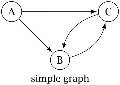
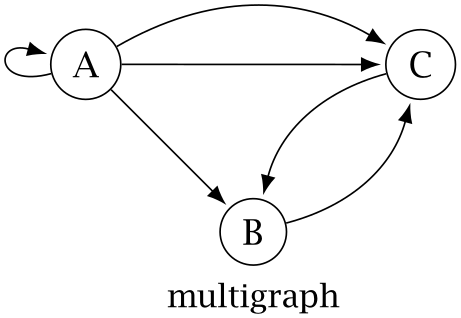
Box 7.1: Simple Graphs and Multigraphs Graph theory distinguishes between simple graphs and multigraphs, which both consist of nodes and edges but differ in the kinds of edges they allow. Here is an example:

(-tikz- diagram) (-tikz- diagram)

The left image shows a simple graph and the right image a multigraph. The difference between the two is that only multigraphs are allowed to have self-loops (here, from A back to itself) and multiple edges between the same pair of nodes (here, from A to C).

Simple graphs are easier to model and easier to process algorithmically, but there are many situations where the added flexibility of multigraphs is required. Even though we will be mostly concerned with simple graphs in this book, many of the ideas and algorithms we will discuss readily generalize to multigraphs.

The neighbors() method shown in in Listing 7.4 computes the neighbors of a given node by trying all the different ways of filling and emptying the jugs. The method first extracts the two decimal digits from node and stores them in large and small. It then computes the amount of water that can be transferred from the large to the small jug largeToSmall and from the small to the large jug smallToLarge. Afterwards the neighbors of node can be computed using the rules discussed above. We store the result in a set data structure to get rid of all potential duplicates and remove the current node itself before returning it to ensure that no node is its own neighbor. (The remove() method does nothing if node isn’t contained in the set, so we can call it unconditionally.)

Listing 7.4ch7 / DieHardGraph

@Override
public Iterable<String> neighbors(String node) {
    int large = Integer.parseInt(node.substring(0, 1));
    int small = Integer.parseInt(node.substring(1, 2));
    int largeToSmall = Math.min(large, 3 - small);
    int smallToLarge = Math.min(5 - large, small);
    var n = new HashSet<String>();
    n.add(makeNode(5, small));
    n.add(makeNode(0, small));
    n.add(makeNode(large, 3));
    n.add(makeNode(large, 0));
    n.add(makeNode(large - largeToSmall, small + largeToSmall));
    n.add(makeNode(large + smallToLarge, small - smallToLarge));
    n.remove(node);
    return n;
}

If we want to compute the neighbors of node \(30\), for example, we first create an instance of DieHardGraph, and then call its neighbors() method:

var graph = new DieHardGraph();
System.out.println(graph.neighbors("30"));

The output is

[00, 33, 03, 50]

which agrees with the list of neighbors shown in Fig. 7.1. In fact, we can reconstruct the entirety of Fig. 7.1 by repeatedly computing lists of neighbors and exploring newly found ones; we will study the resulting algorithm in the following section.

Exercises

Exercise 7.1.The diagram of die-hard graph in Fig. 7.2 doesn’t show the eight interior nodes named 11, 12, …, 42. How are these missing nodes connected to the rest of the graph?

Exercise 7.2.Sketch the die-hard graph that results when the large jug holds 2 gallons and the small jug 1. Can you construct a path through this graph that starts and ends at the same node and visits every other node exactly once? (Such a path is called a Hamiltonian cycle.)