8 Sokoban and Path Finding

\(\newcommand{\footnotename}{footnote}\) \(\def \LWRfootnote {1}\) \(\newcommand {\footnote }[2][\LWRfootnote ]{{}^{\mathrm {#1}}}\) \(\newcommand {\footnotemark }[1][\LWRfootnote ]{{}^{\mathrm {#1}}}\) \(\let \LWRorighspace \hspace \) \(\renewcommand {\hspace }{\ifstar \LWRorighspace \LWRorighspace }\) \(\newcommand {\TextOrMath }[2]{#2}\) \(\newcommand {\mathnormal }[1]{{#1}}\) \(\newcommand \ensuremath [1]{#1}\) \(\newcommand {\LWRframebox }[2][]{\fbox {#2}} \newcommand {\framebox }[1][]{\LWRframebox } \) \(\newcommand {\setlength }[2]{}\) \(\newcommand {\addtolength }[2]{}\) \(\newcommand {\setcounter }[2]{}\) \(\newcommand {\addtocounter }[2]{}\) \(\newcommand {\arabic }[1]{}\) \(\newcommand {\number }[1]{}\) \(\newcommand {\noalign }[1]{\text {#1}\notag \\}\) \(\newcommand {\cline }[1]{}\) \(\newcommand {\directlua }[1]{\text {(directlua)}}\) \(\newcommand {\luatexdirectlua }[1]{\text {(directlua)}}\) \(\newcommand {\protect }{}\) \(\def \LWRabsorbnumber #1 {}\) \(\def \LWRabsorbquotenumber "#1 {}\) \(\newcommand {\LWRabsorboption }[1][]{}\) \(\newcommand {\LWRabsorbtwooptions }[1][]{\LWRabsorboption }\) \(\def \mathchar {\ifnextchar "\LWRabsorbquotenumber \LWRabsorbnumber }\) \(\def \mathcode #1={\mathchar }\) \(\let \delcode \mathcode \) \(\let \delimiter \mathchar \) \(\def \oe {\unicode {x0153}}\) \(\def \OE {\unicode {x0152}}\) \(\def \ae {\unicode {x00E6}}\) \(\def \AE {\unicode {x00C6}}\) \(\def \aa {\unicode {x00E5}}\) \(\def \AA {\unicode {x00C5}}\) \(\def \o {\unicode {x00F8}}\) \(\def \O {\unicode {x00D8}}\) \(\def \l {\unicode {x0142}}\) \(\def \L {\unicode {x0141}}\) \(\def \ss {\unicode {x00DF}}\) \(\def \SS {\unicode {x1E9E}}\) \(\def \dag {\unicode {x2020}}\) \(\def \ddag {\unicode {x2021}}\) \(\def \P {\unicode {x00B6}}\) \(\def \copyright {\unicode {x00A9}}\) \(\def \pounds {\unicode {x00A3}}\) \(\let \LWRref \ref \) \(\renewcommand {\ref }{\ifstar \LWRref \LWRref }\) \( \newcommand {\multicolumn }[3]{#3}\) \(\require {textcomp}\) \(\newcommand {\intertext }[1]{\text {#1}\notag \\}\) \(\let \Hat \hat \) \(\let \Check \check \) \(\let \Tilde \tilde \) \(\let \Acute \acute \) \(\let \Grave \grave \) \(\let \Dot \dot \) \(\let \Ddot \ddot \) \(\let \Breve \breve \) \(\let \Bar \bar \) \(\let \Vec \vec \) \(\renewcommand {\vec }{\boldsymbol }\) \(\newcommand {\Edge }{\ensuremath {\,\textemdash \,}}\) \(\newcommand \Const [1]{\text {\textsf {#1}}}\) \(\DeclareMathOperator {\lerp }{lerp}\) \(\DeclareMathOperator {\bitlen }{bitlen}\) \(\DeclareMathOperator {\sign }{sign}\) \(\newcommand {\I }{\mathrm {i}}\) \(\newcommand \AND {\mathbin {\&}}\) \(\newcommand \OR {\mathbin {|}}\) \(\newcommand \XOR {\mathbin {{}^{\wedge }}}\) \(\newcommand \shl {\ll }\) \(\newcommand \shr {\ggg }\) \(\newcommand \asr {\gg }\) \(\newcommand \NOT {\ensuremath {\mathord {\sim }}}\) \(\newcommand {\isep }{\mathrel {{.}\,{.}}}\) \(\newcommand {\Id }[1]{\mathit {#1}}\) \(\newcommand {\const }[1]{\mathsf {#1}}\) \(\newcommand {\algorithmname }[1]{\text {\textsc {#1}}}\) \(\newcommand {\bits }[1]{\text {#1}}\) \(\newcommand {\hexa }[1]{\mathtt {0x#1}}\) \(\newcommand {\num }[1]{#1}\) \(\newcommand {\qed }{\quad \square }\) \(\newcommand {\idiv }[2]{\lfloor #1/#2\rfloor }\) \(\newcommand \attribdot {\ensuremath {\mkern 1.5mu.\mkern 1.5mu}}\) \(\newcommand \attribxr [2]{#1\attribdot \text {#2}}\) \(\newcommand \attribir [2]{\Id {#1}\attribdot \text {#2}}\) \(\newcommand \attribii [2]{\Id {#1}\attribdot \Id {#2}}\) \(\newcommand \textsc [1]{#1}\) \(\require {colortbl}\) \(\let \LWRorigcolumncolor \columncolor \) \(\renewcommand {\columncolor }[2][named]{\LWRorigcolumncolor [#1]{#2}\LWRabsorbtwooptions }\) \(\let \LWRorigrowcolor \rowcolor \) \(\renewcommand {\rowcolor }[2][named]{\LWRorigrowcolor [#1]{#2}\LWRabsorbtwooptions }\) \(\let \LWRorigcellcolor \cellcolor \) \(\renewcommand {\cellcolor }[2][named]{\LWRorigcellcolor [#1]{#2}\LWRabsorbtwooptions }\) \(\newcommand {\tcbset }[1]{}\) \(\newcommand {\tcbsetforeverylayer }[1]{}\) \(\newcommand {\tcbox }[2][]{\boxed {\text {#2}}}\) \(\newcommand {\tcboxfit }[2][]{\boxed {#2}}\) \(\newcommand {\tcblower }{}\) \(\newcommand {\tcbline }{}\) \(\newcommand {\tcbtitle }{}\) \(\newcommand {\tcbsubtitle [2][]{\mathrm {#2}}}\) \(\newcommand {\tcboxmath }[2][]{\boxed {#2}}\) \(\newcommand {\tcbhighmath }[2][]{\boxed {#2}}\) \(\newcommand {\toprule }[1][]{\hline }\) \(\let \midrule \toprule \) \(\let \bottomrule \toprule \) \(\def \LWRbooktabscmidruleparen (#1)#2{}\) \(\newcommand {\LWRbooktabscmidrulenoparen }[1]{}\) \(\newcommand {\cmidrule }[1][]{\ifnextchar (\LWRbooktabscmidruleparen \LWRbooktabscmidrulenoparen }\) \(\newcommand {\morecmidrules }{}\) \(\newcommand {\specialrule }[3]{\hline }\) \(\newcommand {\addlinespace }[1][]{}\) \(\newcommand {\LWRsubmultirow }[2][]{#2}\) \(\newcommand {\LWRmultirow }[2][]{\LWRsubmultirow }\) \(\newcommand {\multirow }[2][]{\LWRmultirow }\) \(\newcommand {\mrowcell }{}\) \(\newcommand {\mcolrowcell }{}\) \(\newcommand {\STneed }[1]{}\) \(\newcommand {\LWRldelimtwo }[1][]{\text {#1}~\LWRbigdelim }\) \(\newcommand {\LWRldelimone }[2][]{\LWRldelimtwo }\) \(\def \ldelim #1#2{\def \LWRbigdelim {#1}\LWRldelimone }\) \(\newcommand {\LWRrdelimtwo }[1][]{\LWRbigdelim ~\text {#1}}\) \(\newcommand {\LWRrdelimone }[2][]{\LWRrdelimtwo }\) \(\def \rdelim #1#2{\def \LWRbigdelim {#1}\LWRrdelimone }\) \(\let \symnormal \mathit \) \(\let \symliteral \mathrm \) \(\let \symbb \mathbb \) \(\let \symbbit \mathbb \) \(\let \symcal \mathcal \) \(\let \symscr \mathscr \) \(\let \symfrak \mathfrak \) \(\let \symsfup \mathsf \) \(\let \symsfit \mathit \) \(\let \symbfsf \mathbf \) \(\let \symbfup \mathbf \) \(\newcommand {\symbfit }[1]{\boldsymbol {#1}}\) \(\let \symbfcal \mathcal \) \(\let \symbfscr \mathscr \) \(\let \symbffrak \mathfrak \) \(\let \symbfsfup \mathbf \) \(\newcommand {\symbfsfit }[1]{\boldsymbol {#1}}\) \(\let \symup \mathrm \) \(\let \symbf \mathbf \) \(\let \symit \mathit \) \(\let \symsf \symsfit \) \(\let \symtt \mathtt \) \(\let \symbffrac \mathbffrac \) \(\newcommand {\mathfence }[1]{\mathord {#1}}\) \(\newcommand {\mathover }[1]{#1}\) \(\newcommand {\mathunder }[1]{#1}\) \(\newcommand {\mathaccent }[1]{#1}\) \(\newcommand {\mathbotaccent }[1]{#1}\) \(\newcommand {\mathalpha }[1]{\mathord {#1}}\) \(\def\Alpha{\unicode{x1D6E2}}\) \(\def\Beta{\unicode{x1D6E3}}\) \(\def\Gamma{\unicode{x1D6E4}}\) \(\def\Digamma{\mathit{\unicode{x03DC}}}\) \(\def\Delta{\unicode{x1D6E5}}\) \(\def\Epsilon{\unicode{x1D6E6}}\) \(\def\Zeta{\unicode{x1D6E7}}\) \(\def\Eta{\unicode{x1D6E8}}\) \(\def\Theta{\unicode{x1D6E9}}\) \(\def\Vartheta{\unicode{x1D6F3}}\) \(\def\Iota{\unicode{x1D6EA}}\) \(\def\Kappa{\unicode{x1D6EB}}\) \(\def\Lambda{\unicode{x1D6EC}}\) \(\def\Mu{\unicode{x1D6ED}}\) \(\def\Nu{\unicode{x1D6EE}}\) \(\def\Xi{\unicode{x1D6EF}}\) \(\def\Omicron{\unicode{x1D6F0}}\) \(\def\Pi{\unicode{x1D6F1}}\) \(\def\Rho{\unicode{x1D6F2}}\) \(\def\Sigma{\unicode{x1D6F4}}\) \(\def\Tau{\unicode{x1D6F5}}\) \(\def\Upsilon{\unicode{x1D6F6}}\) \(\def\Phi{\unicode{x1D6F7}}\) \(\def\Chi{\unicode{x1D6F8}}\) \(\def\Psi{\unicode{x1D6F9}}\) \(\def\Omega{\unicode{x1D6FA}}\) \(\def\alpha{\unicode{x1D6FC}}\) \(\def\beta{\unicode{x1D6FD}}\) \(\def\varbeta{\unicode{x03D0}}\) \(\def\gamma{\unicode{x1D6FE}}\) \(\def\digamma{\mathit{\unicode{x03DD}}}\) \(\def\delta{\unicode{x1D6FF}}\) \(\def\epsilon{\unicode{x1D716}}\) \(\def\varepsilon{\unicode{x1D700}}\) \(\def\zeta{\unicode{x1D701}}\) \(\def\eta{\unicode{x1D702}}\) \(\def\theta{\unicode{x1D703}}\) \(\def\vartheta{\unicode{x1D717}}\) \(\def\iota{\unicode{x1D704}}\) \(\def\kappa{\unicode{x1D705}}\) \(\def\varkappa{\unicode{x1D718}}\) \(\def\lambda{\unicode{x1D706}}\) \(\def\mu{\unicode{x1D707}}\) \(\def\nu{\unicode{x1D708}}\) \(\def\xi{\unicode{x1D709}}\) \(\def\omicron{\unicode{x1D70A}}\) \(\def\pi{\unicode{x1D70B}}\) \(\def\varpi{\unicode{x1D71B}}\) \(\def\rho{\unicode{x1D70C}}\) \(\def\varrho{\unicode{x1D71A}}\) \(\def\sigma{\unicode{x1D70E}}\) \(\def\varsigma{\unicode{x1D70D}}\) \(\def\tau{\unicode{x1D70F}}\) \(\def\upsilon{\unicode{x1D710}}\) \(\def\phi{\unicode{x1D719}}\) \(\def\varphi{\unicode{x1D711}}\) \(\def\chi{\unicode{x1D712}}\) \(\def\psi{\unicode{x1D713}}\) \(\def\omega{\unicode{x1D714}}\) \(\def\upAlpha{\unicode{x0391}}\) \(\def\upBeta{\unicode{x0392}}\) \(\def\upGamma{\unicode{x0393}}\) \(\def\upDigamma{\unicode{x03DC}}\) \(\def\upDelta{\unicode{x0394}}\) \(\def\upEpsilon{\unicode{x0395}}\) \(\def\upZeta{\unicode{x0396}}\) \(\def\upEta{\unicode{x0397}}\) \(\def\upTheta{\unicode{x0398}}\) \(\def\upVartheta{\unicode{x03F4}}\) \(\def\upIota{\unicode{x0399}}\) \(\def\upKappa{\unicode{x039A}}\) \(\def\upLambda{\unicode{x039B}}\) \(\def\upMu{\unicode{x039C}}\) \(\def\upNu{\unicode{x039D}}\) \(\def\upXi{\unicode{x039E}}\) \(\def\upOmicron{\unicode{x039F}}\) \(\def\upPi{\unicode{x03A0}}\) \(\def\upVarpi{\unicode{x03D6}}\) \(\def\upRho{\unicode{x03A1}}\) \(\def\upSigma{\unicode{x03A3}}\) \(\def\upTau{\unicode{x03A4}}\) \(\def\upUpsilon{\unicode{x03A5}}\) \(\def\upPhi{\unicode{x03A6}}\) \(\def\upChi{\unicode{x03A7}}\) \(\def\upPsi{\unicode{x03A8}}\) \(\def\upOmega{\unicode{x03A9}}\) \(\def\itAlpha{\unicode{x1D6E2}}\) \(\def\itBeta{\unicode{x1D6E3}}\) \(\def\itGamma{\unicode{x1D6E4}}\) \(\def\itDigamma{\mathit{\unicode{x03DC}}}\) \(\def\itDelta{\unicode{x1D6E5}}\) \(\def\itEpsilon{\unicode{x1D6E6}}\) \(\def\itZeta{\unicode{x1D6E7}}\) \(\def\itEta{\unicode{x1D6E8}}\) \(\def\itTheta{\unicode{x1D6E9}}\) \(\def\itVartheta{\unicode{x1D6F3}}\) \(\def\itIota{\unicode{x1D6EA}}\) \(\def\itKappa{\unicode{x1D6EB}}\) \(\def\itLambda{\unicode{x1D6EC}}\) \(\def\itMu{\unicode{x1D6ED}}\) \(\def\itNu{\unicode{x1D6EE}}\) \(\def\itXi{\unicode{x1D6EF}}\) \(\def\itOmicron{\unicode{x1D6F0}}\) \(\def\itPi{\unicode{x1D6F1}}\) \(\def\itRho{\unicode{x1D6F2}}\) \(\def\itSigma{\unicode{x1D6F4}}\) \(\def\itTau{\unicode{x1D6F5}}\) \(\def\itUpsilon{\unicode{x1D6F6}}\) \(\def\itPhi{\unicode{x1D6F7}}\) \(\def\itChi{\unicode{x1D6F8}}\) \(\def\itPsi{\unicode{x1D6F9}}\) \(\def\itOmega{\unicode{x1D6FA}}\) \(\def\upalpha{\unicode{x03B1}}\) \(\def\upbeta{\unicode{x03B2}}\) \(\def\upvarbeta{\unicode{x03D0}}\) \(\def\upgamma{\unicode{x03B3}}\) \(\def\updigamma{\unicode{x03DD}}\) \(\def\updelta{\unicode{x03B4}}\) \(\def\upepsilon{\unicode{x03F5}}\) \(\def\upvarepsilon{\unicode{x03B5}}\) \(\def\upzeta{\unicode{x03B6}}\) \(\def\upeta{\unicode{x03B7}}\) \(\def\uptheta{\unicode{x03B8}}\) \(\def\upvartheta{\unicode{x03D1}}\) \(\def\upiota{\unicode{x03B9}}\) \(\def\upkappa{\unicode{x03BA}}\) \(\def\upvarkappa{\unicode{x03F0}}\) \(\def\uplambda{\unicode{x03BB}}\) \(\def\upmu{\unicode{x03BC}}\) \(\def\upnu{\unicode{x03BD}}\) \(\def\upxi{\unicode{x03BE}}\) \(\def\upomicron{\unicode{x03BF}}\) \(\def\uppi{\unicode{x03C0}}\) \(\def\upvarpi{\unicode{x03D6}}\) \(\def\uprho{\unicode{x03C1}}\) \(\def\upvarrho{\unicode{x03F1}}\) \(\def\upsigma{\unicode{x03C3}}\) \(\def\upvarsigma{\unicode{x03C2}}\) \(\def\uptau{\unicode{x03C4}}\) \(\def\upupsilon{\unicode{x03C5}}\) \(\def\upphi{\unicode{x03D5}}\) \(\def\upvarphi{\unicode{x03C6}}\) \(\def\upchi{\unicode{x03C7}}\) \(\def\uppsi{\unicode{x03C8}}\) \(\def\upomega{\unicode{x03C9}}\) \(\def\italpha{\unicode{x1D6FC}}\) \(\def\itbeta{\unicode{x1D6FD}}\) \(\def\itvarbeta{\unicode{x03D0}}\) \(\def\itgamma{\unicode{x1D6FE}}\) \(\def\itdigamma{\mathit{\unicode{x03DD}}}\) \(\def\itdelta{\unicode{x1D6FF}}\) \(\def\itepsilon{\unicode{x1D716}}\) \(\def\itvarepsilon{\unicode{x1D700}}\) \(\def\itzeta{\unicode{x1D701}}\) \(\def\iteta{\unicode{x1D702}}\) \(\def\ittheta{\unicode{x1D703}}\) \(\def\itvartheta{\unicode{x1D717}}\) \(\def\itiota{\unicode{x1D704}}\) \(\def\itkappa{\unicode{x1D705}}\) \(\def\itvarkappa{\unicode{x1D718}}\) \(\def\itlambda{\unicode{x1D706}}\) \(\def\itmu{\unicode{x1D707}}\) \(\def\itnu{\unicode{x1D708}}\) \(\def\itxi{\unicode{x1D709}}\) \(\def\itomicron{\unicode{x1D70A}}\) \(\def\itpi{\unicode{x1D70B}}\) \(\def\itvarpi{\unicode{x1D71B}}\) \(\def\itrho{\unicode{x1D70C}}\) \(\def\itvarrho{\unicode{x1D71A}}\) \(\def\itsigma{\unicode{x1D70E}}\) \(\def\itvarsigma{\unicode{x1D70D}}\) \(\def\ittau{\unicode{x1D70F}}\) \(\def\itupsilon{\unicode{x1D710}}\) \(\def\itphi{\unicode{x1D719}}\) \(\def\itvarphi{\unicode{x1D711}}\) \(\def\itchi{\unicode{x1D712}}\) \(\def\itpsi{\unicode{x1D713}}\) \(\def\itomega{\unicode{x1D714}}\) \(\let \lparen (\) \(\let \rparen )\) \(\newcommand {\cuberoot }[1]{\,{}^3\!\!\sqrt {#1}}\,\) \(\newcommand {\fourthroot }[1]{\,{}^4\!\!\sqrt {#1}}\,\) \(\newcommand {\longdivision }[1]{\mathord {\unicode {x027CC}#1}}\) \(\newcommand {\mathcomma }{,}\) \(\newcommand {\mathcolon }{:}\) \(\newcommand {\mathsemicolon }{;}\) \(\newcommand {\overbracket }[1]{\mathinner {\overline {\ulcorner {#1}\urcorner }}}\) \(\newcommand {\underbracket }[1]{\mathinner {\underline {\llcorner {#1}\lrcorner }}}\) \(\newcommand {\overbar }[1]{\mathord {#1\unicode {x00305}}}\) \(\newcommand {\ovhook }[1]{\mathord {#1\unicode {x00309}}}\) \(\newcommand {\ocirc }[1]{\mathord {#1\unicode {x0030A}}}\) \(\newcommand {\candra }[1]{\mathord {#1\unicode {x00310}}}\) \(\newcommand {\oturnedcomma }[1]{\mathord {#1\unicode {x00312}}}\) \(\newcommand {\ocommatopright }[1]{\mathord {#1\unicode {x00315}}}\) \(\newcommand {\droang }[1]{\mathord {#1\unicode {x0031A}}}\) \(\newcommand {\leftharpoonaccent }[1]{\mathord {#1\unicode {x020D0}}}\) \(\newcommand {\rightharpoonaccent }[1]{\mathord {#1\unicode {x020D1}}}\) \(\newcommand {\vertoverlay }[1]{\mathord {#1\unicode {x020D2}}}\) \(\newcommand {\leftarrowaccent }[1]{\mathord {#1\unicode {x020D0}}}\) \(\newcommand {\annuity }[1]{\mathord {#1\unicode {x020E7}}}\) \(\newcommand {\widebridgeabove }[1]{\mathord {#1\unicode {x020E9}}}\) \(\newcommand {\asteraccent }[1]{\mathord {#1\unicode {x020F0}}}\) \(\newcommand {\threeunderdot }[1]{\mathord {#1\unicode {x020E8}}}\) \(\newcommand {\Bbbsum }{\mathop {\unicode {x2140}}\limits }\) \(\newcommand {\oiint }{\mathop {\unicode {x222F}}\limits }\) \(\newcommand {\oiiint }{\mathop {\unicode {x2230}}\limits }\) \(\newcommand {\intclockwise }{\mathop {\unicode {x2231}}\limits }\) \(\newcommand {\ointclockwise }{\mathop {\unicode {x2232}}\limits }\) \(\newcommand {\ointctrclockwise }{\mathop {\unicode {x2233}}\limits }\) \(\newcommand {\varointclockwise }{\mathop {\unicode {x2232}}\limits }\) \(\newcommand {\leftouterjoin }{\mathop {\unicode {x27D5}}\limits }\) \(\newcommand {\rightouterjoin }{\mathop {\unicode {x27D6}}\limits }\) \(\newcommand {\fullouterjoin }{\mathop {\unicode {x27D7}}\limits }\) \(\newcommand {\bigbot }{\mathop {\unicode {x27D8}}\limits }\) \(\newcommand {\bigtop }{\mathop {\unicode {x27D9}}\limits }\) \(\newcommand {\xsol }{\mathop {\unicode {x29F8}}\limits }\) \(\newcommand {\xbsol }{\mathop {\unicode {x29F9}}\limits }\) \(\newcommand {\bigcupdot }{\mathop {\unicode {x2A03}}\limits }\) \(\newcommand {\bigsqcap }{\mathop {\unicode {x2A05}}\limits }\) \(\newcommand {\conjquant }{\mathop {\unicode {x2A07}}\limits }\) \(\newcommand {\disjquant }{\mathop {\unicode {x2A08}}\limits }\) \(\newcommand {\bigtimes }{\mathop {\unicode {x2A09}}\limits }\) \(\newcommand {\modtwosum }{\mathop {\unicode {x2A0A}}\limits }\) \(\newcommand {\sumint }{\mathop {\unicode {x2A0B}}\limits }\) \(\newcommand {\intbar }{\mathop {\unicode {x2A0D}}\limits }\) \(\newcommand {\intBar }{\mathop {\unicode {x2A0E}}\limits }\) \(\newcommand {\fint }{\mathop {\unicode {x2A0F}}\limits }\) \(\newcommand {\cirfnint }{\mathop {\unicode {x2A10}}\limits }\) \(\newcommand {\awint }{\mathop {\unicode {x2A11}}\limits }\) \(\newcommand {\rppolint }{\mathop {\unicode {x2A12}}\limits }\) \(\newcommand {\scpolint }{\mathop {\unicode {x2A13}}\limits }\) \(\newcommand {\npolint }{\mathop {\unicode {x2A14}}\limits }\) \(\newcommand {\pointint }{\mathop {\unicode {x2A15}}\limits }\) \(\newcommand {\sqint }{\mathop {\unicode {x2A16}}\limits }\) \(\newcommand {\intlarhk }{\mathop {\unicode {x2A17}}\limits }\) \(\newcommand {\intx }{\mathop {\unicode {x2A18}}\limits }\) \(\newcommand {\intcap }{\mathop {\unicode {x2A19}}\limits }\) \(\newcommand {\intcup }{\mathop {\unicode {x2A1A}}\limits }\) \(\newcommand {\upint }{\mathop {\unicode {x2A1B}}\limits }\) \(\newcommand {\lowint }{\mathop {\unicode {x2A1C}}\limits }\) \(\newcommand {\bigtriangleleft }{\mathop {\unicode {x2A1E}}\limits }\) \(\newcommand {\zcmp }{\mathop {\unicode {x2A1F}}\limits }\) \(\newcommand {\zpipe }{\mathop {\unicode {x2A20}}\limits }\) \(\newcommand {\zproject }{\mathop {\unicode {x2A21}}\limits }\) \(\newcommand {\biginterleave }{\mathop {\unicode {x2AFC}}\limits }\) \(\newcommand {\bigtalloblong }{\mathop {\unicode {x2AFF}}\limits }\) \(\newcommand {\arabicmaj }{\mathop {\unicode {x1EEF0}}\limits }\) \(\newcommand {\arabichad }{\mathop {\unicode {x1EEF1}}\limits }\)

8.6 Dijkstra’s Algorithm

To find the shortest path in a weighted graph, we can use an algorithm known as Dijkstra’s algorithm, named after the Dutch computer scientist Edsger W. Dijkstra. Dijkstra’s algorithm works similar to breadth-first search: starting at a particular node \(S\) of a weighted graph, it visits all reachable nodes in the order of increasing distance from \(S\).

To illustrate how Dijkstra’s algorithm works, consider the simple weighted graph shown in Fig. 8.7. It’s easy to determine the shortest paths from S to all the other nodes by hand: The shortest path to B is \(\text {S}\to \text {B}\) (length 1), the one to C is \(\text {S}\to \text {B}\to \text {C}\) (length 4), the one to A is \(\text {S}\to \text {B}\to \text {A}\) (length 5), and the one to D is \(\text {S}\to \text {B}\to \text {D}\) (length 6). When traversing this graph starting at S, Dijkstra’s algorithm visits the nodes in this order: S, B, C, A, D.

Figure 8.7 A simple weighted graph.

The main idea behind Dijkstra’s algorithm is to maintain a list of nodes that have already been discovered but still need to be explored in more detail. You will recall that this is the same idea that underlies breadth-first search, but in the absence of edge weights we could simply visit the nodes in the order they were discovered and store the list of unexplored nodes in a queue. This is no longer possible when the edges are weighted because the order in which we discover nodes doesn’t always match the order in which we need to visit them. For example, in Fig. 8.7 node A is discovered immediately since it is a direct neighbor of the starting node S, but it is visited after B and C because it is farther away from S.

We can solve this problem by replacing the queue used in breadth-first search with a list of nodes that we keep sorted by their distance from the start. Figure 8.8 illustrates how we can use such a data structure to traverse the graph from Fig. 8.7. Initially, the list of unexplored nodes contains just the starting node S whose distance is obviously 0. In the first step, we visit S and add its two neighbors to the unexplored list, sorted by their distance from S. In each of the following steps, unexplored is updated by removing the first node and adding all or some of its neighbors. In Step 2 we reach node B, which tells us that that B’s distance from S is 1. Three other nodes are reachable from B: node A at total distance 9, node C at total distance 4, and node D at total distance 6. We discard the new path to A since we already discovered a shorter route in the first step, but we add the new nodes C and D to unexplored. In Step 3 we visit C and discover yet another path that leads to A. This path has a total weight of \(5\) and is therefore shorter than the existing path to A, so we update unexplored with the new distance. The last two steps visit A and D and add no new nodes to unexplored.

.
Figure 8.8 Dijkstra’s algorithm visits all nodes that are reachable from the start S in the order of increasing distance. To do this, the algorithm maintains a list of unexplored nodes sorted by their distance from S and visits the nearest unexplored node in each step.

The performance of Dijkstra’s algorithm depends on the data structure that is used to store the list of unexplored nodes. The data structure that is most commonly used for this purpose is the priority queue, which associates a numeric priority with every element of the queue. Priority queues typically provide the following operations:

  • \(\attribir {pq}{isEmpty}()\): Return true if there are no elements in the queue.

  • \(\attribir {pq}{insert}(u, p)\): Add a new element \(u\) with associated priority \(p\) to the queue.

  • \(\attribir {pq}{extractMin}()\): Remove the element with the smallest associated priority from pq and return it.

  • \(\attribir {pq}{decreaseKey}(u, p)\): For an element \(u\) that is already in the queue, reduce its priority to \(p\) and adjust its position in the queue.

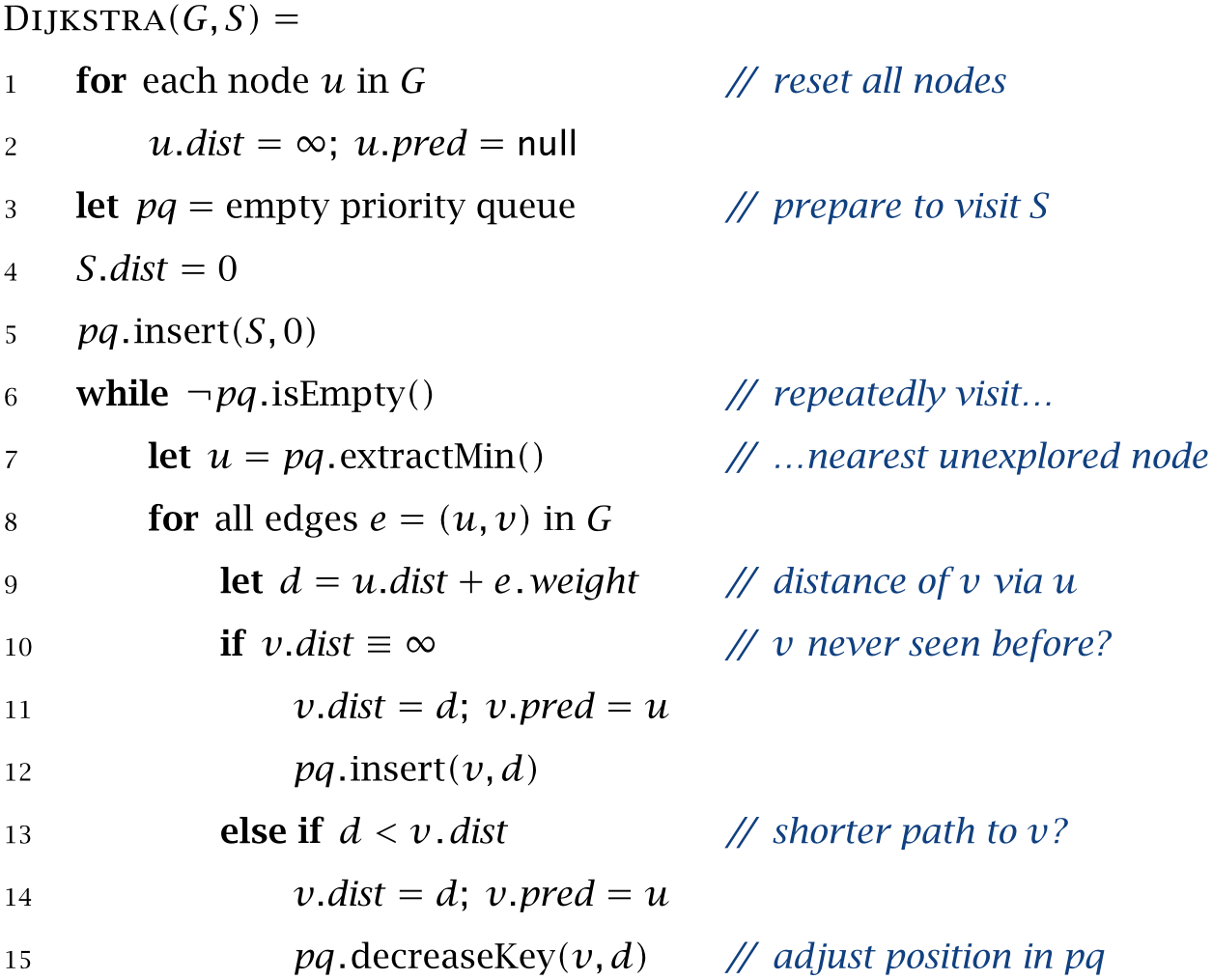
Algorithm 8.1

Dijkstra’s algorithm. Given a weighted graph \(G\) with nonnegative weights and a single node \(S\), determine the shortest paths from \(S\) to every reachable node in \(G\). After the algorithm has completed, the dist field of a node indicates its distance from \(S\) and the pred field is the predecessor along the corresponding shortest path.

(image)

Using such a priority queue, we can describe Dijkstra’s algorithm as shown in Algorithm 8.1. We assume that every node has two fields that can be used to store the algorithm’s output: \(n.\Id {dist}\) for the shortest distance from the start \(S\) to \(n\) and \(n.\Id {pred}\) for the predecessor along the shortest path. At the start of the algorithm, we reset the dist and pred fields of all nodes and then initialize the algorithm by adding \(S\) to the priority queue and setting its dist field to 0. We then repeatedly remove the nearest unexplored node from pq and inspect all its neighbors. For each neighbor \(v\) we distinguish between two conditions. If we haven’t encountered \(v\) before (its dist field is \(\infty \)) we use \(\mathrm {insert}()\) to add it to pq. Otherwise, if the new path to \(v\) via \(u\) is shorter than the one we have found before, we update its dist and pred fields and use \(\mathrm {decreaseKey}()\) to move \(v\) closer to the front of pq.

After the algorithm has finished, we can examine the dist and pred fields to find the shortest path from \(S\) to each node in the graph. If \(n.\Id {dist}\) is \(\infty \), the node hasn’t been reached and no shortest path exists. Otherwise, \(n.\Id {dist}\) is the length of the shortest path, and we can find the nodes on this path by following the pred nodes back to the start.

Implementing Dijkstra’s Algorithm

Let’s now turn to the problem of implementing Dijkstra’s algorithm. Similar to the version of breadth-first search we discussed in Section 7.3, we will store the shortest paths from the starting node as a tree of path segments that link to their predecessors. As before, we define a record that implements the BasicPath interface, but since we are now dealing with paths in a weighted graph, we add a new integer field totalWeight that stores the path’s weighted length from the start. The resulting WeightedPath type is shown in Listing 8.17.

Listing 8.17ch8 / WeightedPath

// Data type for representing paths through weighted graphs.
public record WeightedPath<N>(
        N node, WeightedPath<N> predecessor, int totalWeight)
        implements BasicPath<N> {
}

We implement Dijkstra’s algorithm not as a static function but as a class that stores the algorithm’s state in a handful of fields (Listing 8.18):

  • The graph field is the graph that is being traversed.

  • The dist field corresponds to the dist attribute in Algorithm 8.1 and holds the weighted distance of every visited node from the start.

  • The unexplored field replaces the pq data structure in Algorithm 8.1 and maintains a priority queue of incomplete paths that still need to be explored.

  • The result field is a table that stores the shortest paths to every visited node.

Listing 8.18ch8 / Dijkstra

// Implementation of Dijkstra's algorithm for weighted graphs.
public class Dijkstra<N> {
    private final WeightedGraph<N> graph;
    private final Map<N, Integer> dist = new HashMap<>();
    private final PriorityQueue<WeightedPath<N>> unexplored;
    private final Map<N, WeightedPath<N>> result = new HashMap<>();

    // ...
}

In the pseudocode of Algorithm 8.1, most of the algorithm’s state was stored in two attributes dist and pred that we associated with each node — why do we use different data structures here? One reason is technical: If we want to implement the algorithm generically, we cannot assume that the node type N contains two fields dist and link that we can use for bookkeeping. The only requirement is that we can use N as the key type in a hash table.

The constructor Dijkstra() in Listing 8.19 takes a graph and a starting node as arguments and initializes the algorithm’s data structures. The priority queue for unexplored is initialized using a comparator object that determines how the elements are sorted. Here, the expression

Comparator.comparingInt(WeightedPath::totalWeight)

returns a function that compares two WeightedPath objects by their totalWeight fields, which ensures that the path segment at the front of unexplored is the one with the smallest value of totalWeight. In Algorithm 8.1 we used a loop to reset the dist and pred fields of all nodes before the start of the algorithm; this isn’t necessary here because dist and result are initialized to empty hash tables.

Listing 8.19ch8 / Dijkstra

private Dijkstra(WeightedGraph<N> graph, N start) {
    this.graph = graph;
    unexplored = new PriorityQueue<>(
            Comparator.comparingInt(WeightedPath::totalWeight));
    dist.put(start, 0);
    unexplored.add(new WeightedPath<>(start, null, 0));
}

The main part of Dijkstra’s algorithm repeats the following three steps as long as there are entries in unexplored:

  • 1. Extract the nearest unexplored node from the queue.

  • 2. Check whether it has any undiscovered neighbors or neighbors that can now be reached more quickly.

  • 3. Update the priority queue if that’s the case.

These steps are performed by the nextNode() method shown in Listing 8.20. The implementation differs from the description in Algorithm 8.1 in one crucial respect: If a shorter path to a previously discovered node is found (newDist < oldDist), we don’t update the priority of the existing entry in unexplored but instead add a new entry. This change is necessary because the PriorityQueue class doesn’t support the decreaseKey() operation.

Listing 8.20ch8 / Dijkstra

// Process and return the nearest unexplored node.
private N nextNode() {
    while (!unexplored.isEmpty()) {
        WeightedPath<N> path = unexplored.remove();
        N node = path.node();
        if (result.putIfAbsent(node, path) != null)
            continue;  // skip nodes that were reached before
        for (var edge : graph.edges(node)) {
            int newDist = path.totalWeight() + edge.weight();
            int oldDist = dist.getOrDefault(edge.target(), -1);
            if (oldDist == -1 || newDist < oldDist) {
                dist.put(edge.target(), newDist);
                unexplored.add(
                        new WeightedPath<>(edge.target(), path, newDist));
            }
        }
        return node;
    }
    return null;
}

As a result, unexplored can now contain multiple paths to the same node. The following if statement at the start of the loop ensures that no node is visited more than once:

if (result.putIfAbsent(node, path) != null)
    continue;  // skip nodes that were reached before

The call to putIfAbsent() stores the shortest path to the current node in result, but only the first time this node is encountered. If result already contains an entry for node, we know that the current path must be longer than the one discovered earlier and ignore it.

Finally, we implement two variations of Dijkstra’s algorithm using nextNode() (Listing 8.21). The first is traverse(), which visits every node that is reachable from start and returns a map that contains the shortest path to each of them. The second method shortestPath() works similarly but uses an additional Predicate to stop at the first node that satisfies a certain condition. The method returns either the path to this node or null if no suitable node was found.

Listing 8.21ch8 / Dijkstra

// Visit all nodes reachable from 'start' and return the
// shortest paths.
public static <N> Map<N, WeightedPath<N>> traverse(
        WeightedGraph<N> graph, N start) {
    var dijkstra = new Dijkstra<>(graph, start);
    while (dijkstra.nextNode() != null) {
    }
    return dijkstra.result;
}

// Find the shortest path from 'start' to the nearest node
// that satisfies 'condition'.
public static <N> WeightedPath<N> shortestPath(
        WeightedGraph<N> graph, N start, Predicate<N> condition) {
    var dijkstra = new Dijkstra<>(graph, start);
    while (true) {
        N node = dijkstra.nextNode();
        if (node == null)
            return null;
        if (condition.test(node))
            return dijkstra.result.get(node);
    }
}
Solving Sokoban using the Fewest Steps

With Dijkstra’s algorithm in hand, we can now finally solve our original problem of finding the solution of a given Sokoban level that requires the fewest number of steps. To do this, we first construct the weighted push graph and then search for the shortest path from the starting configuration to any game state that solves the level:

WeightedPath<GameState> path = Dijkstra.shortestPath(
        new WeightedPushGraph(level),
        new GameState(level),
        gameState -> gameState.allCratesOnGoals(level));
System.out.printf("Pushes: %d%n", path.length());
System.out.printf("Steps: %d%n", path.totalWeight());
System.out.println(SokobanSolver.compressMoves(
        SokobanSolver.computeSteps(level, path.toNodeList())));

This outputs the following solution, which requires 230 steps and again 97 pushes — that’s 32 fewer steps than in the solution we found in Section 8.4:

Pushes: 97
Steps: 230
u3l3uLUllDll3dr12R
13lulld14R
7l3ululldDDuull3dr10RurD
7l3ulL3urDDll3Duull3dr10RdRRlU
7l3uL3ull5Duull3dr10RuRRlD
7l3ulLul3Duull3dr10RdRUluR

As before, we have added line breaks to the output to indicate when a crate has reached the goal area. It’s worth trying this solution yourself: Even though most steps are obvious and either move the worker (or a crate) from one side of the level to the other, the final steps on each line, which arrange the crates in the goal area, are surprisingly elegant.

Exercises

Exercise 8.8.A square in a Sokoban level is called dead if there is no way to push a crate from this square to any of the goals.

  • a) Consider the level shown in the following image, which has two goals in the upper right. Which squares in this level are dead?

  • b) Develop an algorithm that computes all dead positions in a Sokoban level.