☰

4 Recursive Curves

\(\newcommand{\footnotename}{footnote}\) \(\def \LWRfootnote {1}\) \(\newcommand {\footnote }[2][\LWRfootnote ]{{}^{\mathrm {#1}}}\) \(\newcommand {\footnotemark }[1][\LWRfootnote ]{{}^{\mathrm {#1}}}\) \(\let \LWRorighspace \hspace \) \(\renewcommand {\hspace }{\ifstar \LWRorighspace \LWRorighspace }\) \(\newcommand {\TextOrMath }[2]{#2}\) \(\newcommand {\mathnormal }[1]{{#1}}\) \(\newcommand \ensuremath [1]{#1}\) \(\newcommand {\LWRframebox }[2][]{\fbox {#2}} \newcommand {\framebox }[1][]{\LWRframebox } \) \(\newcommand {\setlength }[2]{}\) \(\newcommand {\addtolength }[2]{}\) \(\newcommand {\setcounter }[2]{}\) \(\newcommand {\addtocounter }[2]{}\) \(\newcommand {\arabic }[1]{}\) \(\newcommand {\number }[1]{}\) \(\newcommand {\noalign }[1]{\text {#1}\notag \\}\) \(\newcommand {\cline }[1]{}\) \(\newcommand {\directlua }[1]{\text {(directlua)}}\) \(\newcommand {\luatexdirectlua }[1]{\text {(directlua)}}\) \(\newcommand {\protect }{}\) \(\def \LWRabsorbnumber #1 {}\) \(\def \LWRabsorbquotenumber "#1 {}\) \(\newcommand {\LWRabsorboption }[1][]{}\) \(\newcommand {\LWRabsorbtwooptions }[1][]{\LWRabsorboption }\) \(\def \mathchar {\ifnextchar "\LWRabsorbquotenumber \LWRabsorbnumber }\) \(\def \mathcode #1={\mathchar }\) \(\let \delcode \mathcode \) \(\let \delimiter \mathchar \) \(\def \oe {\unicode {x0153}}\) \(\def \OE {\unicode {x0152}}\) \(\def \ae {\unicode {x00E6}}\) \(\def \AE {\unicode {x00C6}}\) \(\def \aa {\unicode {x00E5}}\) \(\def \AA {\unicode {x00C5}}\) \(\def \o {\unicode {x00F8}}\) \(\def \O {\unicode {x00D8}}\) \(\def \l {\unicode {x0142}}\) \(\def \L {\unicode {x0141}}\) \(\def \ss {\unicode {x00DF}}\) \(\def \SS {\unicode {x1E9E}}\) \(\def \dag {\unicode {x2020}}\) \(\def \ddag {\unicode {x2021}}\) \(\def \P {\unicode {x00B6}}\) \(\def \copyright {\unicode {x00A9}}\) \(\def \pounds {\unicode {x00A3}}\) \(\let \LWRref \ref \) \(\renewcommand {\ref }{\ifstar \LWRref \LWRref }\) \( \newcommand {\multicolumn }[3]{#3}\) \(\require {textcomp}\) \(\newcommand {\intertext }[1]{\text {#1}\notag \\}\) \(\let \Hat \hat \) \(\let \Check \check \) \(\let \Tilde \tilde \) \(\let \Acute \acute \) \(\let \Grave \grave \) \(\let \Dot \dot \) \(\let \Ddot \ddot \) \(\let \Breve \breve \) \(\let \Bar \bar \) \(\let \Vec \vec \) \(\renewcommand {\vec }{\boldsymbol }\) \(\newcommand {\Edge }{\ensuremath {\,\textemdash \,}}\) \(\newcommand \Const [1]{\text {\textsf {#1}}}\) \(\DeclareMathOperator {\lerp }{lerp}\) \(\DeclareMathOperator {\bitlen }{bitlen}\) \(\DeclareMathOperator {\sign }{sign}\) \(\newcommand {\I }{\mathrm {i}}\) \(\newcommand \AND {\mathbin {\&}}\) \(\newcommand \OR {\mathbin {|}}\) \(\newcommand \XOR {\mathbin {{}^{\wedge }}}\) \(\newcommand \shl {\ll }\) \(\newcommand \shr {\ggg }\) \(\newcommand \asr {\gg }\) \(\newcommand \NOT {\ensuremath {\mathord {\sim }}}\) \(\newcommand {\isep }{\mathrel {{.}\,{.}}}\) \(\newcommand {\Id }[1]{\mathit {#1}}\) \(\newcommand {\const }[1]{\mathsf {#1}}\) \(\newcommand {\algorithmname }[1]{\text {\textsc {#1}}}\) \(\newcommand {\bits }[1]{\text {#1}}\) \(\newcommand {\hexa }[1]{\mathtt {0x#1}}\) \(\newcommand {\num }[1]{#1}\) \(\newcommand {\qed }{\quad \square }\) \(\newcommand {\idiv }[2]{\lfloor #1/#2\rfloor }\) \(\newcommand \attribdot {\ensuremath {\mkern 1.5mu.\mkern 1.5mu}}\) \(\newcommand \attribxr [2]{#1\attribdot \text {#2}}\) \(\newcommand \attribir [2]{\Id {#1}\attribdot \text {#2}}\) \(\newcommand \attribii [2]{\Id {#1}\attribdot \Id {#2}}\) \(\newcommand \textsc [1]{#1}\) \(\require {colortbl}\) \(\let \LWRorigcolumncolor \columncolor \) \(\renewcommand {\columncolor }[2][named]{\LWRorigcolumncolor [#1]{#2}\LWRabsorbtwooptions }\) \(\let \LWRorigrowcolor \rowcolor \) \(\renewcommand {\rowcolor }[2][named]{\LWRorigrowcolor [#1]{#2}\LWRabsorbtwooptions }\) \(\let \LWRorigcellcolor \cellcolor \) \(\renewcommand {\cellcolor }[2][named]{\LWRorigcellcolor [#1]{#2}\LWRabsorbtwooptions }\) \(\newcommand {\tcbset }[1]{}\) \(\newcommand {\tcbsetforeverylayer }[1]{}\) \(\newcommand {\tcbox }[2][]{\boxed {\text {#2}}}\) \(\newcommand {\tcboxfit }[2][]{\boxed {#2}}\) \(\newcommand {\tcblower }{}\) \(\newcommand {\tcbline }{}\) \(\newcommand {\tcbtitle }{}\) \(\newcommand {\tcbsubtitle [2][]{\mathrm {#2}}}\) \(\newcommand {\tcboxmath }[2][]{\boxed {#2}}\) \(\newcommand {\tcbhighmath }[2][]{\boxed {#2}}\) \(\newcommand {\toprule }[1][]{\hline }\) \(\let \midrule \toprule \) \(\let \bottomrule \toprule \) \(\def \LWRbooktabscmidruleparen (#1)#2{}\) \(\newcommand {\LWRbooktabscmidrulenoparen }[1]{}\) \(\newcommand {\cmidrule }[1][]{\ifnextchar (\LWRbooktabscmidruleparen \LWRbooktabscmidrulenoparen }\) \(\newcommand {\morecmidrules }{}\) \(\newcommand {\specialrule }[3]{\hline }\) \(\newcommand {\addlinespace }[1][]{}\) \(\newcommand {\LWRsubmultirow }[2][]{#2}\) \(\newcommand {\LWRmultirow }[2][]{\LWRsubmultirow }\) \(\newcommand {\multirow }[2][]{\LWRmultirow }\) \(\newcommand {\mrowcell }{}\) \(\newcommand {\mcolrowcell }{}\) \(\newcommand {\STneed }[1]{}\) \(\newcommand {\LWRldelimtwo }[1][]{\text {#1}~\LWRbigdelim }\) \(\newcommand {\LWRldelimone }[2][]{\LWRldelimtwo }\) \(\def \ldelim #1#2{\def \LWRbigdelim {#1}\LWRldelimone }\) \(\newcommand {\LWRrdelimtwo }[1][]{\LWRbigdelim ~\text {#1}}\) \(\newcommand {\LWRrdelimone }[2][]{\LWRrdelimtwo }\) \(\def \rdelim #1#2{\def \LWRbigdelim {#1}\LWRrdelimone }\) \(\let \symnormal \mathit \) \(\let \symliteral \mathrm \) \(\let \symbb \mathbb \) \(\let \symbbit \mathbb \) \(\let \symcal \mathcal \) \(\let \symscr \mathscr \) \(\let \symfrak \mathfrak \) \(\let \symsfup \mathsf \) \(\let \symsfit \mathit \) \(\let \symbfsf \mathbf \) \(\let \symbfup \mathbf \) \(\newcommand {\symbfit }[1]{\boldsymbol {#1}}\) \(\let \symbfcal \mathcal \) \(\let \symbfscr \mathscr \) \(\let \symbffrak \mathfrak \) \(\let \symbfsfup \mathbf \) \(\newcommand {\symbfsfit }[1]{\boldsymbol {#1}}\) \(\let \symup \mathrm \) \(\let \symbf \mathbf \) \(\let \symit \mathit \) \(\let \symsf \symsfit \) \(\let \symtt \mathtt \) \(\let \symbffrac \mathbffrac \) \(\newcommand {\mathfence }[1]{\mathord {#1}}\) \(\newcommand {\mathover }[1]{#1}\) \(\newcommand {\mathunder }[1]{#1}\) \(\newcommand {\mathaccent }[1]{#1}\) \(\newcommand {\mathbotaccent }[1]{#1}\) \(\newcommand {\mathalpha }[1]{\mathord {#1}}\) \(\def\Alpha{\unicode{x1D6E2}}\) \(\def\Beta{\unicode{x1D6E3}}\) \(\def\Gamma{\unicode{x1D6E4}}\) \(\def\Digamma{\mathit{\unicode{x03DC}}}\) \(\def\Delta{\unicode{x1D6E5}}\) \(\def\Epsilon{\unicode{x1D6E6}}\) \(\def\Zeta{\unicode{x1D6E7}}\) \(\def\Eta{\unicode{x1D6E8}}\) \(\def\Theta{\unicode{x1D6E9}}\) \(\def\Vartheta{\unicode{x1D6F3}}\) \(\def\Iota{\unicode{x1D6EA}}\) \(\def\Kappa{\unicode{x1D6EB}}\) \(\def\Lambda{\unicode{x1D6EC}}\) \(\def\Mu{\unicode{x1D6ED}}\) \(\def\Nu{\unicode{x1D6EE}}\) \(\def\Xi{\unicode{x1D6EF}}\) \(\def\Omicron{\unicode{x1D6F0}}\) \(\def\Pi{\unicode{x1D6F1}}\) \(\def\Rho{\unicode{x1D6F2}}\) \(\def\Sigma{\unicode{x1D6F4}}\) \(\def\Tau{\unicode{x1D6F5}}\) \(\def\Upsilon{\unicode{x1D6F6}}\) \(\def\Phi{\unicode{x1D6F7}}\) \(\def\Chi{\unicode{x1D6F8}}\) \(\def\Psi{\unicode{x1D6F9}}\) \(\def\Omega{\unicode{x1D6FA}}\) \(\def\alpha{\unicode{x1D6FC}}\) \(\def\beta{\unicode{x1D6FD}}\) \(\def\varbeta{\unicode{x03D0}}\) \(\def\gamma{\unicode{x1D6FE}}\) \(\def\digamma{\mathit{\unicode{x03DD}}}\) \(\def\delta{\unicode{x1D6FF}}\) \(\def\epsilon{\unicode{x1D716}}\) \(\def\varepsilon{\unicode{x1D700}}\) \(\def\zeta{\unicode{x1D701}}\) \(\def\eta{\unicode{x1D702}}\) \(\def\theta{\unicode{x1D703}}\) \(\def\vartheta{\unicode{x1D717}}\) \(\def\iota{\unicode{x1D704}}\) \(\def\kappa{\unicode{x1D705}}\) \(\def\varkappa{\unicode{x1D718}}\) \(\def\lambda{\unicode{x1D706}}\) \(\def\mu{\unicode{x1D707}}\) \(\def\nu{\unicode{x1D708}}\) \(\def\xi{\unicode{x1D709}}\) \(\def\omicron{\unicode{x1D70A}}\) \(\def\pi{\unicode{x1D70B}}\) \(\def\varpi{\unicode{x1D71B}}\) \(\def\rho{\unicode{x1D70C}}\) \(\def\varrho{\unicode{x1D71A}}\) \(\def\sigma{\unicode{x1D70E}}\) \(\def\varsigma{\unicode{x1D70D}}\) \(\def\tau{\unicode{x1D70F}}\) \(\def\upsilon{\unicode{x1D710}}\) \(\def\phi{\unicode{x1D719}}\) \(\def\varphi{\unicode{x1D711}}\) \(\def\chi{\unicode{x1D712}}\) \(\def\psi{\unicode{x1D713}}\) \(\def\omega{\unicode{x1D714}}\) \(\def\upAlpha{\unicode{x0391}}\) \(\def\upBeta{\unicode{x0392}}\) \(\def\upGamma{\unicode{x0393}}\) \(\def\upDigamma{\unicode{x03DC}}\) \(\def\upDelta{\unicode{x0394}}\) \(\def\upEpsilon{\unicode{x0395}}\) \(\def\upZeta{\unicode{x0396}}\) \(\def\upEta{\unicode{x0397}}\) \(\def\upTheta{\unicode{x0398}}\) \(\def\upVartheta{\unicode{x03F4}}\) \(\def\upIota{\unicode{x0399}}\) \(\def\upKappa{\unicode{x039A}}\) \(\def\upLambda{\unicode{x039B}}\) \(\def\upMu{\unicode{x039C}}\) \(\def\upNu{\unicode{x039D}}\) \(\def\upXi{\unicode{x039E}}\) \(\def\upOmicron{\unicode{x039F}}\) \(\def\upPi{\unicode{x03A0}}\) \(\def\upVarpi{\unicode{x03D6}}\) \(\def\upRho{\unicode{x03A1}}\) \(\def\upSigma{\unicode{x03A3}}\) \(\def\upTau{\unicode{x03A4}}\) \(\def\upUpsilon{\unicode{x03A5}}\) \(\def\upPhi{\unicode{x03A6}}\) \(\def\upChi{\unicode{x03A7}}\) \(\def\upPsi{\unicode{x03A8}}\) \(\def\upOmega{\unicode{x03A9}}\) \(\def\itAlpha{\unicode{x1D6E2}}\) \(\def\itBeta{\unicode{x1D6E3}}\) \(\def\itGamma{\unicode{x1D6E4}}\) \(\def\itDigamma{\mathit{\unicode{x03DC}}}\) \(\def\itDelta{\unicode{x1D6E5}}\) \(\def\itEpsilon{\unicode{x1D6E6}}\) \(\def\itZeta{\unicode{x1D6E7}}\) \(\def\itEta{\unicode{x1D6E8}}\) \(\def\itTheta{\unicode{x1D6E9}}\) \(\def\itVartheta{\unicode{x1D6F3}}\) \(\def\itIota{\unicode{x1D6EA}}\) \(\def\itKappa{\unicode{x1D6EB}}\) \(\def\itLambda{\unicode{x1D6EC}}\) \(\def\itMu{\unicode{x1D6ED}}\) \(\def\itNu{\unicode{x1D6EE}}\) \(\def\itXi{\unicode{x1D6EF}}\) \(\def\itOmicron{\unicode{x1D6F0}}\) \(\def\itPi{\unicode{x1D6F1}}\) \(\def\itRho{\unicode{x1D6F2}}\) \(\def\itSigma{\unicode{x1D6F4}}\) \(\def\itTau{\unicode{x1D6F5}}\) \(\def\itUpsilon{\unicode{x1D6F6}}\) \(\def\itPhi{\unicode{x1D6F7}}\) \(\def\itChi{\unicode{x1D6F8}}\) \(\def\itPsi{\unicode{x1D6F9}}\) \(\def\itOmega{\unicode{x1D6FA}}\) \(\def\upalpha{\unicode{x03B1}}\) \(\def\upbeta{\unicode{x03B2}}\) \(\def\upvarbeta{\unicode{x03D0}}\) \(\def\upgamma{\unicode{x03B3}}\) \(\def\updigamma{\unicode{x03DD}}\) \(\def\updelta{\unicode{x03B4}}\) \(\def\upepsilon{\unicode{x03F5}}\) \(\def\upvarepsilon{\unicode{x03B5}}\) \(\def\upzeta{\unicode{x03B6}}\) \(\def\upeta{\unicode{x03B7}}\) \(\def\uptheta{\unicode{x03B8}}\) \(\def\upvartheta{\unicode{x03D1}}\) \(\def\upiota{\unicode{x03B9}}\) \(\def\upkappa{\unicode{x03BA}}\) \(\def\upvarkappa{\unicode{x03F0}}\) \(\def\uplambda{\unicode{x03BB}}\) \(\def\upmu{\unicode{x03BC}}\) \(\def\upnu{\unicode{x03BD}}\) \(\def\upxi{\unicode{x03BE}}\) \(\def\upomicron{\unicode{x03BF}}\) \(\def\uppi{\unicode{x03C0}}\) \(\def\upvarpi{\unicode{x03D6}}\) \(\def\uprho{\unicode{x03C1}}\) \(\def\upvarrho{\unicode{x03F1}}\) \(\def\upsigma{\unicode{x03C3}}\) \(\def\upvarsigma{\unicode{x03C2}}\) \(\def\uptau{\unicode{x03C4}}\) \(\def\upupsilon{\unicode{x03C5}}\) \(\def\upphi{\unicode{x03D5}}\) \(\def\upvarphi{\unicode{x03C6}}\) \(\def\upchi{\unicode{x03C7}}\) \(\def\uppsi{\unicode{x03C8}}\) \(\def\upomega{\unicode{x03C9}}\) \(\def\italpha{\unicode{x1D6FC}}\) \(\def\itbeta{\unicode{x1D6FD}}\) \(\def\itvarbeta{\unicode{x03D0}}\) \(\def\itgamma{\unicode{x1D6FE}}\) \(\def\itdigamma{\mathit{\unicode{x03DD}}}\) \(\def\itdelta{\unicode{x1D6FF}}\) \(\def\itepsilon{\unicode{x1D716}}\) \(\def\itvarepsilon{\unicode{x1D700}}\) \(\def\itzeta{\unicode{x1D701}}\) \(\def\iteta{\unicode{x1D702}}\) \(\def\ittheta{\unicode{x1D703}}\) \(\def\itvartheta{\unicode{x1D717}}\) \(\def\itiota{\unicode{x1D704}}\) \(\def\itkappa{\unicode{x1D705}}\) \(\def\itvarkappa{\unicode{x1D718}}\) \(\def\itlambda{\unicode{x1D706}}\) \(\def\itmu{\unicode{x1D707}}\) \(\def\itnu{\unicode{x1D708}}\) \(\def\itxi{\unicode{x1D709}}\) \(\def\itomicron{\unicode{x1D70A}}\) \(\def\itpi{\unicode{x1D70B}}\) \(\def\itvarpi{\unicode{x1D71B}}\) \(\def\itrho{\unicode{x1D70C}}\) \(\def\itvarrho{\unicode{x1D71A}}\) \(\def\itsigma{\unicode{x1D70E}}\) \(\def\itvarsigma{\unicode{x1D70D}}\) \(\def\ittau{\unicode{x1D70F}}\) \(\def\itupsilon{\unicode{x1D710}}\) \(\def\itphi{\unicode{x1D719}}\) \(\def\itvarphi{\unicode{x1D711}}\) \(\def\itchi{\unicode{x1D712}}\) \(\def\itpsi{\unicode{x1D713}}\) \(\def\itomega{\unicode{x1D714}}\) \(\let \lparen (\) \(\let \rparen )\) \(\newcommand {\cuberoot }[1]{\,{}^3\!\!\sqrt {#1}}\,\) \(\newcommand {\fourthroot }[1]{\,{}^4\!\!\sqrt {#1}}\,\) \(\newcommand {\longdivision }[1]{\mathord {\unicode {x027CC}#1}}\) \(\newcommand {\mathcomma }{,}\) \(\newcommand {\mathcolon }{:}\) \(\newcommand {\mathsemicolon }{;}\) \(\newcommand {\overbracket }[1]{\mathinner {\overline {\ulcorner {#1}\urcorner }}}\) \(\newcommand {\underbracket }[1]{\mathinner {\underline {\llcorner {#1}\lrcorner }}}\) \(\newcommand {\overbar }[1]{\mathord {#1\unicode {x00305}}}\) \(\newcommand {\ovhook }[1]{\mathord {#1\unicode {x00309}}}\) \(\newcommand {\ocirc }[1]{\mathord {#1\unicode {x0030A}}}\) \(\newcommand {\candra }[1]{\mathord {#1\unicode {x00310}}}\) \(\newcommand {\oturnedcomma }[1]{\mathord {#1\unicode {x00312}}}\) \(\newcommand {\ocommatopright }[1]{\mathord {#1\unicode {x00315}}}\) \(\newcommand {\droang }[1]{\mathord {#1\unicode {x0031A}}}\) \(\newcommand {\leftharpoonaccent }[1]{\mathord {#1\unicode {x020D0}}}\) \(\newcommand {\rightharpoonaccent }[1]{\mathord {#1\unicode {x020D1}}}\) \(\newcommand {\vertoverlay }[1]{\mathord {#1\unicode {x020D2}}}\) \(\newcommand {\leftarrowaccent }[1]{\mathord {#1\unicode {x020D0}}}\) \(\newcommand {\annuity }[1]{\mathord {#1\unicode {x020E7}}}\) \(\newcommand {\widebridgeabove }[1]{\mathord {#1\unicode {x020E9}}}\) \(\newcommand {\asteraccent }[1]{\mathord {#1\unicode {x020F0}}}\) \(\newcommand {\threeunderdot }[1]{\mathord {#1\unicode {x020E8}}}\) \(\newcommand {\Bbbsum }{\mathop {\unicode {x2140}}\limits }\) \(\newcommand {\oiint }{\mathop {\unicode {x222F}}\limits }\) \(\newcommand {\oiiint }{\mathop {\unicode {x2230}}\limits }\) \(\newcommand {\intclockwise }{\mathop {\unicode {x2231}}\limits }\) \(\newcommand {\ointclockwise }{\mathop {\unicode {x2232}}\limits }\) \(\newcommand {\ointctrclockwise }{\mathop {\unicode {x2233}}\limits }\) \(\newcommand {\varointclockwise }{\mathop {\unicode {x2232}}\limits }\) \(\newcommand {\leftouterjoin }{\mathop {\unicode {x27D5}}\limits }\) \(\newcommand {\rightouterjoin }{\mathop {\unicode {x27D6}}\limits }\) \(\newcommand {\fullouterjoin }{\mathop {\unicode {x27D7}}\limits }\) \(\newcommand {\bigbot }{\mathop {\unicode {x27D8}}\limits }\) \(\newcommand {\bigtop }{\mathop {\unicode {x27D9}}\limits }\) \(\newcommand {\xsol }{\mathop {\unicode {x29F8}}\limits }\) \(\newcommand {\xbsol }{\mathop {\unicode {x29F9}}\limits }\) \(\newcommand {\bigcupdot }{\mathop {\unicode {x2A03}}\limits }\) \(\newcommand {\bigsqcap }{\mathop {\unicode {x2A05}}\limits }\) \(\newcommand {\conjquant }{\mathop {\unicode {x2A07}}\limits }\) \(\newcommand {\disjquant }{\mathop {\unicode {x2A08}}\limits }\) \(\newcommand {\bigtimes }{\mathop {\unicode {x2A09}}\limits }\) \(\newcommand {\modtwosum }{\mathop {\unicode {x2A0A}}\limits }\) \(\newcommand {\sumint }{\mathop {\unicode {x2A0B}}\limits }\) \(\newcommand {\intbar }{\mathop {\unicode {x2A0D}}\limits }\) \(\newcommand {\intBar }{\mathop {\unicode {x2A0E}}\limits }\) \(\newcommand {\fint }{\mathop {\unicode {x2A0F}}\limits }\) \(\newcommand {\cirfnint }{\mathop {\unicode {x2A10}}\limits }\) \(\newcommand {\awint }{\mathop {\unicode {x2A11}}\limits }\) \(\newcommand {\rppolint }{\mathop {\unicode {x2A12}}\limits }\) \(\newcommand {\scpolint }{\mathop {\unicode {x2A13}}\limits }\) \(\newcommand {\npolint }{\mathop {\unicode {x2A14}}\limits }\) \(\newcommand {\pointint }{\mathop {\unicode {x2A15}}\limits }\) \(\newcommand {\sqint }{\mathop {\unicode {x2A16}}\limits }\) \(\newcommand {\intlarhk }{\mathop {\unicode {x2A17}}\limits }\) \(\newcommand {\intx }{\mathop {\unicode {x2A18}}\limits }\) \(\newcommand {\intcap }{\mathop {\unicode {x2A19}}\limits }\) \(\newcommand {\intcup }{\mathop {\unicode {x2A1A}}\limits }\) \(\newcommand {\upint }{\mathop {\unicode {x2A1B}}\limits }\) \(\newcommand {\lowint }{\mathop {\unicode {x2A1C}}\limits }\) \(\newcommand {\bigtriangleleft }{\mathop {\unicode {x2A1E}}\limits }\) \(\newcommand {\zcmp }{\mathop {\unicode {x2A1F}}\limits }\) \(\newcommand {\zpipe }{\mathop {\unicode {x2A20}}\limits }\) \(\newcommand {\zproject }{\mathop {\unicode {x2A21}}\limits }\) \(\newcommand {\biginterleave }{\mathop {\unicode {x2AFC}}\limits }\) \(\newcommand {\bigtalloblong }{\mathop {\unicode {x2AFF}}\limits }\) \(\newcommand {\arabicmaj }{\mathop {\unicode {x1EEF0}}\limits }\) \(\newcommand {\arabichad }{\mathop {\unicode {x1EEF1}}\limits }\)

4.3 De Casteljau’s Algorithm

Bézier curves and Hilbert curves have something important in common: they can both be defined recursively. Similar to the way a Hilbert curve consists of multiple smaller Hilbert curves of lower order, a Bézier curve can be subdivided into multiple smaller Bézier curves with different control points.

One way to perform this subdivision is an elegant algorithm known as de Casteljau’s algorithm. This algorithm constructs points on a Bézier curve geometrically — without evaluating the polynomial in Eq. (4.2) — by repeatedly averaging the four control points \(\vec {p}_0, \dots , \vec {p}_3\). In the first step we take each pair of adjacent control points and compute their average:

\begin{equation*} \vec {q}_0=\frac {\vec {p}_0+\vec {p}_1}{2},\qquad \vec {q}_1=\frac {\vec {p}_1+\vec {p}_2}{2},\qquad \vec {q}_2=\frac {\vec {p}_2+\vec {p}_3}{2}. \end{equation*}

In the second step we average those three points again to obtain two points:

\begin{equation*} \vec {r}_0=\frac {\vec {q}_0+\vec {q}_1}{2},\qquad \vec {r}_1=\frac {\vec {q}_1+\vec {q}_2}{2}. \end{equation*}

And in the last step we average one more time to obtain a single point

\begin{equation*} \vec {s} = \frac {\vec {r}_0 + \vec {r}_1}{2}. \end{equation*}

As illustrated in Fig. 4.6, this final point lies on the Bézier curve; in fact, it is easy to show that we have \(\vec {s}=\vec {B}(1/2)\) (see Exercise 4.8).

Figure 4.6 De Casteljau’s algorithm repeatedly averages the control points of a given Bézier curve to produce a single point \(\vec {s}\) that splits the curve in the middle. The left and right half of the curve are also Bézier curves.

The point \(\vec {s}\) splits the original curve into two halves, \(\vec {B}_1(t)\) and \(\vec {B}_2(t)\), both of which are Bézier curves in their own right. As suggested by Fig. 4.6, the control points of the first half are \(\vec {p}_0\), \(\vec {q}_0\), \(\vec {r}_0\), and \(\vec {s}\), and those of the second half are \(\vec {s}\), \(\vec {r}_1\), \(\vec {q}_2\), and \(\vec {p}_3\), so we have

\begin{equation} \label {eq:beziersplit} \begin{aligned} \vec {B}_1(t) &= (1-t)^3 \vec {p}_0 + 3t(1-t)^2 \vec {q}_0 + 3t^2(1-t)\vec {r}_0 + t^3 \vec {s},\\ \vec {B}_2(t) &= (1-t)^3 \vec {s} + 3t(1-t)^2 \vec {r}_1 + 3t^2(1-t)\vec {q}_2 + t^3 \vec {p}_3. \end {aligned} \end{equation}

The split() method in Listing 4.4 uses this equation to split a given BezierCurve into two halves.

Listing 4.4ch4β€―/β€―BezierCurve

// Split Bézier curve in the middle, producing two smaller curves.
public BezierCurve[] split() {
    Point q0 = mid(p0, p1), q1 = mid(p1, p2), q2 = mid(p2, p3);
    Point r0 = mid(q0, q1), r1 = mid(q1, q2);
    Point s = mid(r0, r1);
    return new BezierCurve[]{
            new BezierCurve(p0, q0, r0, s),
            new BezierCurve(s, r1, q2, p3)};
}

// Compute the midpoint of a and b.
static Point mid(Point a, Point b) {
    return Point.lerp(a, b, 0.5);
}

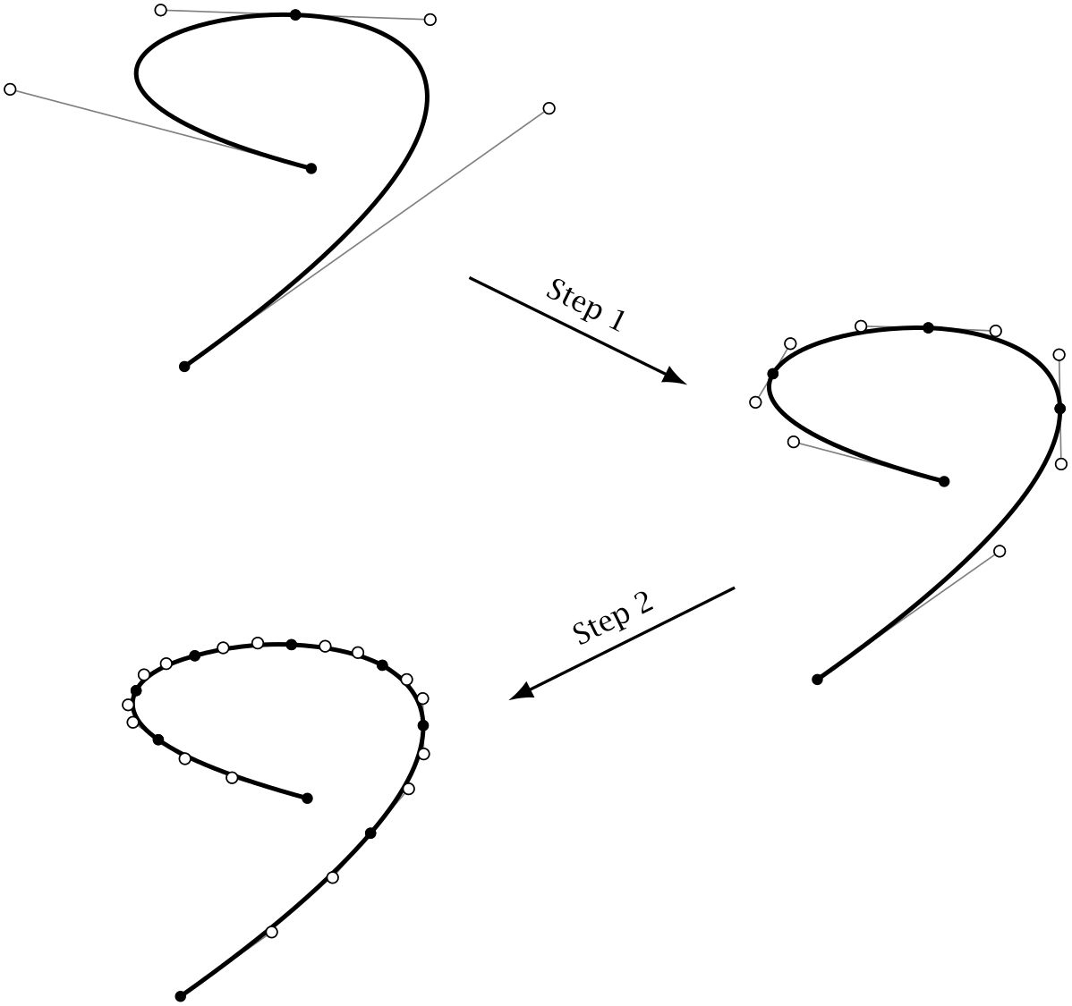
Of course, we can apply de Casteljau’s algorithm repeatedly and thereby subdivide the original Bézier curve into 4, 8, 16, and ultimately as many pieces as we like. This is the essence of de Casteljau’s algorithm: a procedure for splitting Bézier curves into a hierarchy of smaller Bézier curves (Fig. 4.7).

(-tikz- diagram)

Figure 4.7 Repeated application of de Casteljau’s algorithm. Each step produces a finer subdivision by doubling the number of curve segments. Notice also how the control points contract and move towards the curve itself.
Adaptive Subdivision

The main benefit of de Casteljau’s algorithm isn’t that it lets us compute a certain number of points on a Bézier curve — we could already do that before — but that each curve segment it produces is a Bézier curve in its own right. In this section, we first develop a simple test to determine whether a Bézier curve is approximately straight and then use this test guide the subdivision process so that only curve segments that aren’t already straight enough are subdivided further. This idea is known as adaptive subdivision.

How do we test the straightness of a Bézier curve? A simple criterion is based on the following observation: If the inner control points \(\vec {p}_1\) and \(\vec {p}_2\) lie at \(1/3\) and \(2/3\) of the distance between the two end points \(\vec {p}_0\) and \(\vec {p}_3\), it can be shown that the resulting Bézier curve is mathematically identical to a line segment (see Exercise 4.8). We can therefore consider a Bézier curve almost straight if the first control point \(\vec {p}_1\) is close to \(\lerp (\vec {p}_0, \vec {p}_3, 1/3)\) and the second control point \(\vec {p}_2\) is close to \(\lerp (\vec {p}_0, \vec {p}_3, 2/3)\), which means that their distance is less than a given tolerance \(T\):

\begin{equation} \label {eq:bezier:straight} \bigl |\vec {p}_1 - \lerp (\vec {p}_0, \vec {p}_3, 1/3)\bigr | < T \qquad \text {and}\qquad \bigl |\vec {p}_2 - \lerp (\vec {p}_0, \vec {p}_3, 2/3)\bigr | < T. \end{equation}

By setting \(T\) to a sufficiently small value, say, a value that is smaller than the size of a pixel, we can distinguish between curve segments that are visually indistinguishable from a line segment and segments that need further subdivision.

By combining this straightness test with de Casteljau’s subdivision algorithm, we can write a function subdivide() that recursively subdivides a Bézier curve until all segments satisfy the straightness criterion in Eq. (4.6); see Listing 4.5. The parameter tolerance specifies the desired level of straightness and corresponds to the parameter \(T\) in Eq. (4.6). The function produces a sequence of points on the curve and adds them to the final argument result.

Listing 4.5ch4β€―/β€―BezierCurve

// Recursively subdivide curve until all segments are straight.
void subdivide(double tolerance, List<Point> result) {
    if (isStraight(tolerance)) {
        result.add(p3);
    } else {
        BezierCurve[] segments = split();
        segments[0].subdivide(tolerance, result);
        segments[1].subdivide(tolerance, result);
    }
}

boolean isStraight(double tolerance) {
    double d1 = Point.distance(p1, Point.lerp(p0, p3, 1.0 / 3.0));
    double d2 = Point.distance(p2, Point.lerp(p0, p3, 2.0 / 3.0));
    return d1 < tolerance && d2 < tolerance;
}

The function first uses isStraight() to test whether the current curve must be subdivided further. If the current curve segment is sufficiently straight, subdivide() stops the subdivision process and appends the end point of the current segment p3 to the list of points. Otherwise, it splits the curve in half using de Casteljau’s algorithm and recursively calls itself to further subdivide the two halves.

You may be wondering why subdivide() only adds the second end point p3 of each straight segment to result and not the starting point p0. The reason is that adding both points would cause every interior point on the curve to be added twice to result since the end point of the each segment is the starting point of the next. Adding only the second end point solves the problem of duplicates, but it also omits the starting point of the entire curve. This can be easily remedied by manually adding this point right before starting the subdivision process, as shown in Listing 4.6.

Listing 4.6ch4β€―/β€―BezierCurve

public List<Point> draw(double tolerance) {
    List<Point> result = new ArrayList<>();
    result.add(p0);
    subdivide(tolerance, result);
    return result;
}

The images in Fig. 4.8 illustrate how the straightness tolerance influences the final subdivision of a given Bézier curve. For \(T=1\), we obtain four line segments which corresponds to two applications of Casteljau’s algorithm, but as we decrease the value of \(T\), additional points on the curve are generated to produce a finer subdivision. Notice that decreasing the tolerance always produces a refinement of the previous subdivision: More points are added in certain parts of the curve as necessary, but existing points are never removed. It’s also easy to see that the subdivision is indeed adaptive, so the point density is highest in regions where the curve is strongly bent.

Figure 4.8 Adaptive subdivision of Bézier curves. The straightness tolerance T measures how much the curve segments are allowed to deviate from a straight line. Smaller tolerance produces finer subdivisions.

There is one important question we haven’t addressed yet: With this straightness test, can we be sure that the subdivision process always terminates, or are there any Bézier curves that can be subdivided endlessly, without ever being considered straight enough? Fortunately, Bézier curves are sufficiently well-behaved that this cannot happen. Every time we split a Bézier curve into two smaller segments, the control points of the new curves move closer together (and closer to the curve itself) because they are computed by averaging the old control points; this effect can be easily observed in Fig. 4.7. For every fixed tolerance \(T\), the conditions in Eq. (4.6) must therefore be satisfied after a finite number of iterations.

Exercises

\(\star \) Exercise 4.3.How do we prove that the two Bézier curves in Eq. (4.5) together form the original curve \(\vec {B}(t)\)? The key is to realize that the first half of the original curve can be written as \(\vec {B}(t/2)\) and the second half as \(\vec {B}(t/2 + 1/2)\). We then have to show that

\begin{equation*} \vec {B}(t/2) = \vec {B}_1(t)\qquad \text {and}\qquad \vec {B}(t/2+1/2) = \vec {B}_2(t). \end{equation*}

Complete the proof by expanding both sides of these equations using Eq. (4.2) for \(\vec {B}(t)\) and Eq. (4.5) for \(\vec {B}_1(t)\) and \(\vec {B}_2(t)\).

Exercise 4.4.Modify de Casteljau’s algorithm to compute the approximate length of a Bézier curve.