C Answers to Exercises
Chapter 7
Solution to Exercise 7.1
The normal rules for computing neighbors can be used for the interior nodes. Every interior node has exactly six neighbors but no incoming edges. In graph theory, a node with no incoming edges is called a source, so all these nodes are sources.
Solution to Exercise 7.2
The graph looks as follows:
One Hamiltonian cycle is \(00\to {}20\to {}11\to {}21\to {}01\to {}10\to {}00\).
Solution to Exercise 7.3
True. There is always a layer at distance 0 that contains just the starting node.
Solution to Exercise 7.4
Due to the symmetry of the graph, there are just four different eccentricities:
\(\seteqnumber{0}{C.}{5}\)\begin{equation*} \begin{array}{cc} n & \epsilon (n)\\ 00,03,50,53& 7\\ 20,23,30,33& 6\\ 01,02,51,52& 5\\ 10,13,40,43& 4 \end {array} \end{equation*}
Solution to Exercise 7.5
The implementation of printNodes() in Listing C.49 collects the string representation of every node on the path and then joins them into a single string.
Listing C.49ch7 / Path
default String printNodes() {
    var nodeNames = new ArrayList<String>();
    for (N node : toNodeList())
        nodeNames.add(node.toString());
    return String.join(" -> ", nodeNames);
}
JDK: ArrayList, String
•BasicPath: toNodeList()
Solution to Exercise 7.6
a)The problem has two solutions that differ in whether the wolf or the cabbage is transferred in the second step:
-
1. Move the goat to the other shore.
-
2a. Move the wolf and take the goat back on the return trip. Then move the cabbage.
-
2b. Move the cabbage and take the goat back on the return trip. Then move the wolf.
-
3. Move the goat.
b)If we represent this side of the river by 0 and the other side by 1, we can encode the current positions of the wolf, the goat, and the cabbage as a sequence of three digits \(wgc\). There are obviously 8 such states. (The farmer’s position simply alternates between the two sides of the river and is therefore redundant.) We start in the \(000\) state in which the entire party is on this side of the river, and the goal is to transition to the \(111\) state where everyone is on the other side. Every time the farmer ferries one party member across the river, the corresponding digit flips from 0 to 1 or vice versa.
c)Here is an image of the graph corresponding to the wolf-goat-cabbage problem:
If you mirror the graph vertically or horizontally, you obtain the same graph with different labels. The left-right symmetry reflects the fact that it doesn’t matter how we label the banks of the river, and the up-down symmetry the fact that the wolf and the cabbage constrain the problem in the same way: They both cannot be left alone with the goat.
There are two different paths of length 5 from the start 000 to the destination 111, one moving along the top of the graph and the other along the bottom:
\(\seteqnumber{0}{C.}{5}\)\begin{align*} & 000\to {}010\to {}110\to {}100\to {}101\to {}111 && \text {upper path}\\ & 000\to {}010\to {}011\to {}001\to {}101\to {}111 && \text {lower path} \end{align*} The two paths differ mainly in whether the farmer takes the wolf or the cabbage on the second trip.
d)If we are currently in a state \(wgc\), the next state is either \((1-w)gc\), \(w(1-g)c\), or \(wg(1-c)\). The wolf’s digit may only be flipped if the goat and the cabbage are currently on different sides of the river, in other words if \(g\ne c\), and for a similar reason, the cabbage digit may only be flipped if \(w\ne g\); only the goat digit may be flipped at any time, regardless of the other digits. We can therefore transition to a neighboring state under the following conditions:
\(\seteqnumber{0}{C.}{5}\)\begin{equation} \label {eq:wgc} \begin{array}{@{}cc} \text {\emph {neighbor state}} & \text {\emph {condition}}\\ (1-w)gc & g\ne c\\ w(1-g)c & \\ wg(1-c) & w\ne g\\ \end {array} \end{equation}
For instance, in the starting state \(000\), we have both \(g=c\) and \(w=g\), so the first and last conditions are not satisfied and only the goat can be transferred to the other side of the river, which gives us the new state \(010\). For this new state, we have \(g\ne c\) and \(w\ne g\), so we can transition into all three neighboring states \(110\), \(000\), and \(011\). Notice that the second transition leads us back to the original state, which corresponds to the fact that the farmer can always undo her last move.
We can represent each node in the wolf-goat-cabbage graph as a String of binary digits and the entire graph as a class that implements Graph
Listing C.50ch7 / WolfGoatCabbageGraph
public class WolfGoatCabbageGraph implements Graph<String> {
    public List<String> nodes() {
        return List.of("000", "001", "010", "011",
                "100", "101", "110", "111");
    }

    public List<String> neighbors(String state) {
        List<String> neighbors = new ArrayList<>();
        if (state.charAt(1) != state.charAt(2))
            neighbors.add(flipDigit(state, 0));
        neighbors.add(flipDigit(state, 1));
        if (state.charAt(0) != state.charAt(1))
            neighbors.add(flipDigit(state, 2));
        return neighbors;
    }

    private static String flipDigit(String state, int index) {
        return state.substring(0, index)
                + (state.charAt(index) == '0' ? '1' : '0')
                + state.substring(index + 1);
    }
}
Solution to Exercise 7.7
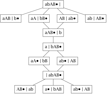
a)If we let the lower-case letters a and b stand for the women and A and B for their husbands, we can write each state of the puzzle as a pair of strings such as “a | bAB•”, where the first string is the group on the left bank, the second string the group on the right, and the position of the boat is indicated by ‘•’. Only six other states are reachable from starting state “abAB• |”:
bAB | a• aAB | b• aA | bB• bB | aA• AB | ab• ab | AB•
Notice that the two states “bAB | a•” and “aAB | b•” are equivalent since one can be obtained from the other by renaming the two couples; similarly, “aA | bB•” is equivalent to “bB | aA•”. If we continue from here, advancing from newly discovered states and combining equivalent ones if possible, we obtain the graph shown in Fig. C.10. It takes five steps to reach the destination “| abAB•”.
b)The JealousCouples.State record in Listing C.51 describes the current state of the puzzle using four values: the position of the boat boatPos and three bit sets that hold the people on the left and right riverbank and the island. We store the bits set in an array of 64-bit integers groups and a normalized version of these sets in normalizedGroups; as we will explain below, these normalized sets allows us to identify puzzle states that are equivalent to states that have already been explored. We omit the implementation of toString(), which prints an instance of State in a format similar to the one discussed in the answer to part (a). To be able to store State objects in hash tables we override equals() and hashCode(); notice that both methods use normalizedGroups instead of groups.
Listing C.51ch7 / JealousCouples
public record State(
        int boatPos,  // location of the boat (0, 1, 2)
        long[] groups,  // bit set of people at each location
        long[] normalizedGroups)  // normalized version of 'groups'
{
    @Override
    public boolean equals(Object obj) {
        return (obj instanceof State state)
                && boatPos == state.boatPos
                && Arrays.equals(normalizedGroups, state.normalizedGroups);
    }

    @Override
    public int hashCode() {
        return Integer.hashCode(boatPos) * 31
                + Arrays.hashCode(normalizedGroups);
    }
}
The puzzle itself can now be modeled as a graph with nodes of type State. This graph has two parameters: the number of couples and a Boolean that indicates whether there is an island (Listing C.52).
Listing C.52ch7 / JealousCouples
public class JealousCouples
        implements Graph<JealousCouples.State> {
    int numCouples;
    int numLocations;

    public JealousCouples(int numCouples, boolean hasIsland) {
        this.numCouples = numCouples;
        this.numLocations = hasIsland ? 3 : 2;
    }

    // ...
}
We allow up to 26 couples and use integers between 0 and 25 for the wives and integers between 26 and 51 for their husbands. The set representation makes it easy to determine whether a particular group provokes no jealousy: That’s the case if the set of women without their partner present is empty (womenAlone == 0) or if no men are present in the first place (men == 0). Both quantities can be computed using bit operations (Listing C.53).
Listing C.53ch7 / JealousCouples
static final int MAX_COUPLES = 26;
static final long WOMEN_MASK = Bits.range(0, MAX_COUPLES);
static final long MEN_MASK =
        Bits.range(MAX_COUPLES, 2 * MAX_COUPLES);

static boolean noJealousy(long group) {
    long men = group & MEN_MASK;
    long women = group & WOMEN_MASK;
    long womenAlone = women & ~(men >>> MAX_COUPLES);
    return womenAlone == 0 || men == 0;
}
•Bits: range()
•JealousCouples
We can now tackle the problem of computing the neighbors of a given State in the puzzle’s graph. Every legal move involves sending one or two people and the boat from its current location to another location. We can therefore construct all potential new states by iterating over all possible destinations and all possible pairs of passengers and keeping only those states that don’t violate the “no jealousy” rule, as shown in Listing C.54. Notice that the innermost loop starts at j = i, so trips in which only a single person uses the boat are also generated.
Listing C.54ch7 / JealousCouples
@Override
public Collection<State> neighbors(State state) {
    var neighbors = new HashSet<State>();
    var here = state.groups[state.boatPos];
    for (int d = 1; d < numLocations; d++) {
        int dest = (state.boatPos + d) % numLocations;
        for (int i : Bits.iterate(here)) {
            for (int j : Bits.iterate(here & Bits.range(i)))
                checkTrip(state, Bits.bits(i, j), dest, neighbors);
        }
    }
    return neighbors;
}
JDK: HashSet
•Bits: bit(), iterate()
•JealousCouples: checkTrip(), State
A trip is allowed only if the new groups at the current location and the destination provoke no jealousy (if this is the case, the group of passengers is guaranteed to provoke no jealousy). The checkTrip() method in Listing C.55 performs the necessary checks and adds a new state to neighbors if successful.
Listing C.55ch7 / JealousCouples
private void checkTrip(State state,
        long passengers, int destination,
        Collection<State> neighbors) {
    long newHere = state.groups[state.boatPos] & ~passengers;
    long newThere = state.groups[destination] | passengers;
    if (noJealousy(newHere) && noJealousy(newThere)) {
        var newGroups = Arrays.copyOf(state.groups, numLocations);
        newGroups[state.boatPos] = newHere;
        newGroups[destination] = newThere;
        neighbors.add(makeState(destination, newGroups));
    }
}
As we noted in the solution of part (a), two puzzle states are equivalent if one can be obtained from the other by renaming the couples. For example, if we already investigated “bB | aA•” there is no need to investigate “aA | bB•” as well because we will only find permutations of previous solutions.
We can identify equivalent states by mapping each state to a unique normalized representative. One way to choose this representative is to reorder the couples in such a way the women appear in alphabetical order when read from left to right. For example, we can normalize “cdC | abAB | D” by performing the substitutions \(\text {c}\to \text {a}\), \(\text {d}\to \text {b}\), \(\text {b}\to \text {c}\), and \(\text {a}\to \text {d}\) (and likewise for the upper-case letters), which gives us the state “abA | cdCD | B” in which the order of the women is “abcd”.
The makeState() method in Listing C.56 performs this normalization by iterating over the women in the three bit sets and assigning each of them (and her husband) a new index based on the order in which she is encountered. The method returns a new State object.
Listing C.56ch7 / JealousCouples
private State makeState(int boat, long[] groups) {
    long[] newGroups = new long[numLocations];
    int newId = 0;
    for (int i = 0; i < numLocations; i++) {
        long women = groups[i] & WOMEN_MASK;
        for (int woman : Bits.iterate(women)) {
            // Assign new ID to woman and her husband
            newGroups[i] |= Bits.bit(newId);
            for (int j = 0; j < groups.length; j++) {
                if (Bits.contains(groups[j], woman + MAX_COUPLES))
                    newGroups[j] |= Bits.bit(newId + MAX_COUPLES);
            }
            newId++;
        }
    }
    return new State(boat, groups, newGroups);
}
•Bits: bit(), contains(), iterate()
•JealousCouples
Using makeState(), we can also construct the starting state and the end state, in which all couples are at either the first or the second location (Listing C.57).
Listing C.57ch7 / JealousCouples
private long everyone() {
    return Bits.range(0, numCouples)
            | Bits.range(MAX_COUPLES, MAX_COUPLES + numCouples);
}

public State start() {
    return makeState(0, new long[]{everyone(), 0L, 0L});
}

public State end() {
    return makeState(1, new long[]{0L, everyone(), 0L});
}
•Bits: range()
•JealousCouples: makeState()
c)If there is an island, the problem has a solution for all \(n\ge 2\). For \(n=2\) and \(n=3\) the solutions are identical to the problem without an island. For \(n\ge 5\) the number of steps is always \(4n+1\); see the article by Pressman and Singmaster [78] for a mathematical proof.
| \(n\) | 2 | 3 | 4 | 5 | 6 | 7 | 8 | 9 | 10 |
| number of trips | 5 | 11 | 16 | 21 | 25 | 29 | 33 | 37 | 41 |
Solution to Exercise 7.8
a)The two problems are closely related since there is a one-to-one correspondence between states of the problem: If \(L\) and \(S\) denote the amount of water in the large and small jug and \(A\) the amount of water in the additional jug, we always have \(A=8-L+S\). Evenly dividing the original amount of water means we are searching for a path from \(A=8,L=0,S=0\) to \(A=4,L=4,S=0\), that is, from the “00” state to the “40” state in the die-hard graph. As we saw in Fig. 7.1, this requires seven steps.
b)The resulting graph is shown in Fig. C.11; the three numbers in the label of each node indicate the amount of water in the three jugs. We start at the node labeled 006 in which all water is in the third jug. As you can see, the overall shape of the graph is similar to the die-hard graph in Fig. 7.2, but restricting the total amount of water renders three of the original nodes in the upper-right corner inaccessible and causes changes to some of the edges. The quickest way to measure four gallons is \(006\to 501\to 231\to 204\), and the trivial solution to dividing the initial six gallons evenly is \(006\to 033\).
c)The implementation in Listing C.58 stores the size of the three jugs in the capacity array and the total amount of water used in totalAmount. The list of nodes computed by nodes() consists of all triples \((x,y,z)\) such that \(x\), \(y\), and \(z\) are below the corresponding capacity and the sum \(x+y+z\) is equal to totalAmount. The neighbors() method computes the neighbors of a state by picking two distinct jugs \(i\) and \(j\) and pouring the contents of \(i\) into \(j\), either until \(i\) is empty or \(j\) is full.
Listing C.58ch7 / ThreeJugProblem
public class ThreeJugProblem implements Graph<List<Integer>> {
    private final int[] capacity;
    private final int totalAmount;

    @Override
    public Iterable<List<Integer>> nodes() {
        var n = new ArrayList<List<Integer>>();
        for (int x = 0; x < capacity[0]; x++) {
            for (int y = 0; y < capacity[1]; y++) {
                int z = totalAmount - x - y;
                if (z >= 0)
                    n.add(List.of(x, y, z));
            }
        }
        return n;
    }

    @Override
    public Iterable<List<Integer>> neighbors(List<Integer> node) {
        var n = new ArrayList<List<Integer>>();
        for (int i = 0; i < 3; i++) {
            for (int j = 0; j < 3; j++) {
                int transfer = Math.min(
                        node.get(i), capacity[j] - node.get(j));
                if (i == j || transfer == 0)
                    continue;
                var neighbor = new ArrayList<>(node);
                neighbor.set(i, neighbor.get(i) - transfer);
                neighbor.set(j, neighbor.get(j) + transfer);
                n.add(neighbor);
            }
        }
        return n;
    }
}
d)The diameter of the graph in Fig. C.11 is \(6\). The two most difficult measuring problems both involve 6 steps, and the corresponding paths are \(006\to 501\to 231\to 204\to 024\to 420\to 402\) and \(303\to 501\to 231\to 204\to 024\to 420\to 402\).
Solution to Exercise 7.9
a)The \(\text {Hanoi}(3)\) and \(\text {Hanoi}(4)\) graphs are shown in Fig. C.12. For large values of \(n\), the graph increasingly looks like the Sierpiński triangle we already met in Section 1.1.
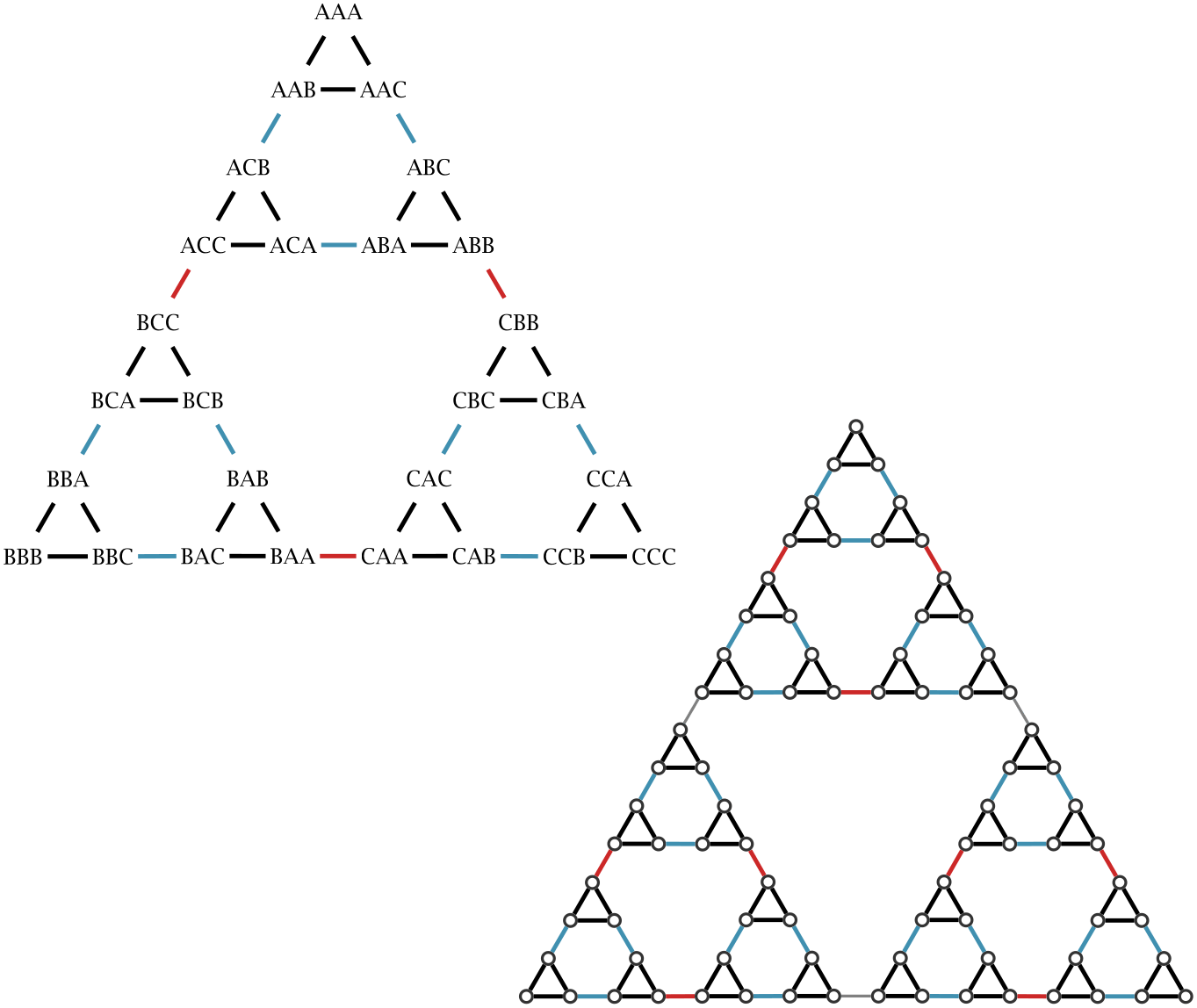
The graph \(\text {Hanoi}(n)\) has \(3^n\) nodes since there are three ways to place largest disk, three ways to place the second-largest disk, and so on. The number of edges \(E_n\) satisfies the following recurrence relation:
\(\seteqnumber{0}{C.}{6}\)\begin{equation} E_0 = 0,\qquad E_n = 3E_{n-1} + 3. \end{equation}
Using induction, it’s easy to prove that \(E_n=(3^{n+1}-3)/2\).
b)Every legal move transfers the topmost disk from one peg to another peg. The labels of neighboring nodes differ in exactly one letter, and the letter that changes in either label is always the rightmost instance of A, B, or C. We can state this mathematically as follows: There is an edge between two nodes \(X\) and \(Y\) if their labels differ in exactly one position \(i\), and if the letter \(X_i\) is the rightmost A, B, or C in \(X\) and the letter \(Y_i\) is the rightmost A, B, or C in \(Y\).
The HanoiGraph class in Listing C.59 uses these conditions to compute the Hanoi graph. The neighbors() method first precomputes an array topDisk that holds the smallest disk on each of the three pegs; the number \(0\) represents the largest disk and \(n-1\) the smallest. If one of the pegs is empty, the corresponding entry in topDisk is set to \(-1\). For example, for the AABAB state, topDisk is {3, 4, -1} since disk 3 is the topmost disk on peg A, disk 4 the topmost disk on peg B, and peg C is empty. Moving a disk from peg to targetPeg is only allowed if topDisk[peg] isn’t \(-1\) and
topDisk[targetPeg] < topDisk[peg]
Notice that this condition also handles the case where the target peg is empty, since in this case topDisk[targetPeg] contains the value \(-1\).
Listing C.59ch7 / HanoiGraph
public record HanoiGraph(int numDisks) implements Graph<String> {
    @Override
    public List<String> neighbors(String state) {
        int[] topDisk = new int[3];
        for (int peg = 0; peg < 3; peg++)
            topDisk[peg] = state.lastIndexOf('A' + peg);
        var neighbors = new ArrayList<String>();
        for (int disk : topDisk) {
            if (disk == -1)
                continue;  // no disk on current peg
            for (int targetPeg = 0; targetPeg < 3; targetPeg++) {
                if (topDisk[targetPeg] < disk) {
                    neighbors.add(state.substring(0, disk)
                            + (char) ('A' + targetPeg)
                            + state.substring(disk + 1));
                }
            }
        }
        return neighbors;
    }
    // ...
}
c)To find the shortest path between two corners of the Hanoi graph, breadth-first search has to visit almost every node of the graph. In contrast, the recursive algorithm in Exercise 3.8 computes the shortest path directly, without wasting time on nodes that don’t lie on the path. Since \(\text {Hanoi}(n)\) has \(3^n\) nodes but its side length is “just” \(2^n\), breadth-first search has to evaluate \((3/2)^n\) times more nodes than the dedicated algorithm — it literally has to work exponentially harder!
d)For \(\text {Hanoi}(2)\), a possible Hamiltonian cycle is
\(\seteqnumber{0}{C.}{7}\)\begin{equation*} \text {AA}\to {}\text {AC}\to {}\text {BC}\to {}\text {BB}\to {}\text {BA}\to {}\text {CA}\to {}\text {CC}\to {}\text {CB}\to {}\text {AB}\to {}\text {AA}. \end{equation*}
Likewise, for \(\text {Hanoi}(3)\) a possible Hamiltonian cycle is
\(\seteqnumber{0}{C.}{7}\)\begin{gather*} \text {ACC}\to {}\text {ACA}\to {}\text {ACB}\to {}\text {AAB}\to {}\text {AAA}\to {}\text {AAC}\to {}\text {ABC}\to {}\text {ABA}\to {}\text {ABB}\to {}\\ \text {CBB}\to {}\text {CBA}\to {}\text {CBC}\to {}\text {CAC}\to {}\text {CAA}\to {}\text {CAB}\to {}\text {CCB}\to {}\text {CCA}\to {}\text {CCC}\to {}\\ \text {BBB}\to {}\text {BBA}\to {}\text {BBC}\to {}\text {BAC}\to {}\text {BAA}\to {}\text {BAB}\to {}\text {BCB}\to {}\text {BCA}\to {}\text {BCC}\to {}\text {ACC}. \end{gather*} Other solutions can be found by reversing these paths or shifting them circularly.
e)First note that every Hanoi graph consists of three smaller Hanoi graphs that are connected at the edges, as shown in Fig. C.13. Let’s say we want to construct a Hamiltonian path \(P_n(A_0, C_0)\) that connects the corners \(A_0\) and \(C_0\) of \(\text {Hanoi}(n)\). We show that this is possible for every value of \(n\). For \(\text {Hanoi}(1)\), the Hamiltonian path simply connects the three corners \(A_0\to {}B_0\to {}C_0\). For \(n>1\), we recursively construct suitable Hamiltonian paths for the three sub-graphs and connect them at the edges:
\(\seteqnumber{0}{C.}{7}\)\begin{equation*} P_n(A_0, C_0) = P_{n-1}(A_0, A_1) \to {} P_{n-1}(B_2, B_1) \to {} P_{n-1}(C_2, C_0). \end{equation*}
It follows by induction that every Hanoi graph contains a Hamiltonian path between any pair of corners.
We can use a similar construction to show that every Hanoi graph also contains a Hamiltonian cycle. Assume we want to construct a Hamiltonian cycle in \(\text {Hanoi}(n)\) that starts and ends at the \(A_2\) node in Fig. C.13. Since the cycle must visit every node exactly once, it must have the following general form:
\(\seteqnumber{0}{C.}{7}\)\begin{equation*} C_n = P_{n-1}(A_2, A_1) \to {} P_{n-1}(B_2, B_1) \to {} P_{n-1}(C_2, C_1) \to {} A_2, \end{equation*}
where each \(P_{n-1}\) is a Hamiltonian path through one of the smaller Hanoi graphs. We just saw that it is always possible to construct the paths \(P_{n-1}\), so there is a Hamiltonian cycle \(C_n\) for every value of \(n\).
Solution to Exercise 7.10
a)If the starting pixel already has the desired color, the algorithm does nothing and returns immediately. Listing C.60 shows an implementation for images of type BufferedImage:
Listing C.60ch7 / FloodFill
record PixelPos(int x, int y) {}

// Fill the region connected to the pixel (startX, startY)
// with a new color. Process one pixel at a time.
public static void floodFill_pixelBased(BufferedImage image,
        int startX, int startY, int fillColor) {
    int startColor = image.getRGB(startX, startY);
    if (image.getRGB(startX, startY) == fillColor)
        return;
    var queue = new ArrayDeque<PixelPos>();
    queue.add(new PixelPos(startX, startY));
    while (!queue.isEmpty()) {
        PixelPos pixelPos = queue.poll();
        int x = pixelPos.x(), y = pixelPos.y();
        image.setRGB(x, y, fillColor);
        if (x > 0 && image.getRGB(x - 1, y) == startColor) {
            queue.add(new PixelPos(x - 1, y));
        }
        if (x < image.getWidth() - 1
                && image.getRGB(x + 1, y) == startColor) {
            queue.add(new PixelPos(x + 1, y));
        }
        if (y > 0 && image.getRGB(x, y - 1) == startColor) {
            queue.add(new PixelPos(x, y - 1));
        }
        if (y < image.getHeight() - 1
                && image.getRGB(x, y + 1) == startColor) {
            queue.add(new PixelPos(x, y + 1));
        }
    }
}
JDK: ArrayDeque, BufferedImage
b)There is a total of eleven spans:
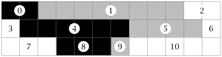
The following spans are adjacent: \(0\Edge {}4\Edge {}8\), \(1\Edge {}5\), \(2\Edge {}6\Edge {}10\), \(3\Edge {}7\).
c)Let’s start with a more detailed description of the span-based flood fill algorithm:
-
• We use a queue to keep track of unprocessed spans. It isn’t necessary to determine the extent of each span in advance. Instead, each entry in the queue can be a single pixel somewhere on the span to be filled.
-
• When processing each span, we first determine its left edge by moving to the left. We then move to the right and replace all pixels on the span with the desired fill color.
-
• While moving right, we inspect the pixels above and below the current pixel and check if they also have the starting color. If they do, they are part of another span that needs to be filled and we add their coordinates to the queue. Only the first pixel of each span above or below should be added to the queue so that each span is processed only once.
Listing C.61 shows an implementation of this idea.
Listing C.61ch7 / FloodFill
// Fill the region connected to the pixel (startX, startY)
// with a new color. Process horizontal spans of pixels.
public static void floodFill_spanBased(
        BufferedImage image, int startX, int startY, int fillColor) {
    int startColor = image.getRGB(startX, startY);
    if (image.getRGB(startX, startY) == fillColor)
        return;
    var queue = new ArrayDeque<PixelPos>();
    queue.add(new PixelPos(startX, startY));
    while (!queue.isEmpty()) {
        PixelPos pixelPos = queue.poll();

        // Move to the start of the current span.
        int x = pixelPos.x();
        int y = pixelPos.y();
        while (x > 0 && image.getRGB(x - 1, y) == startColor)
            x--;

        // Color pixels on this span and find new spans above and below.
        boolean skipSpanAbove = false;
        boolean skipSpanBelow = false;
        while (x < image.getWidth()
                && image.getRGB(x, y) == startColor) {
            image.setRGB(x, y, fillColor);
            boolean matchingColorAbove = y > 0
                    && image.getRGB(x, y - 1) == startColor;
            boolean matchingColorBelow = y < image.getHeight() - 1
                    && image.getRGB(x, y + 1) == startColor;
            if (matchingColorAbove && !skipSpanAbove)
                queue.add(new PixelPos(x, y - 1));
            if (matchingColorBelow && !skipSpanBelow)
                queue.add(new PixelPos(x, y + 1));
            skipSpanAbove = matchingColorAbove;
            skipSpanBelow = matchingColorBelow;
            x++;
        }
    }
}
JDK: ArrayDeque, BufferedImage
•FloodFill: PixelPos