C Answers to Exercises

\(\newcommand{\footnotename}{footnote}\) \(\def \LWRfootnote {1}\) \(\newcommand {\footnote }[2][\LWRfootnote ]{{}^{\mathrm {#1}}}\) \(\newcommand {\footnotemark }[1][\LWRfootnote ]{{}^{\mathrm {#1}}}\) \(\let \LWRorighspace \hspace \) \(\renewcommand {\hspace }{\ifstar \LWRorighspace \LWRorighspace }\) \(\newcommand {\TextOrMath }[2]{#2}\) \(\newcommand {\mathnormal }[1]{{#1}}\) \(\newcommand \ensuremath [1]{#1}\) \(\newcommand {\LWRframebox }[2][]{\fbox {#2}} \newcommand {\framebox }[1][]{\LWRframebox } \) \(\newcommand {\setlength }[2]{}\) \(\newcommand {\addtolength }[2]{}\) \(\newcommand {\setcounter }[2]{}\) \(\newcommand {\addtocounter }[2]{}\) \(\newcommand {\arabic }[1]{}\) \(\newcommand {\number }[1]{}\) \(\newcommand {\noalign }[1]{\text {#1}\notag \\}\) \(\newcommand {\cline }[1]{}\) \(\newcommand {\directlua }[1]{\text {(directlua)}}\) \(\newcommand {\luatexdirectlua }[1]{\text {(directlua)}}\) \(\newcommand {\protect }{}\) \(\def \LWRabsorbnumber #1 {}\) \(\def \LWRabsorbquotenumber "#1 {}\) \(\newcommand {\LWRabsorboption }[1][]{}\) \(\newcommand {\LWRabsorbtwooptions }[1][]{\LWRabsorboption }\) \(\def \mathchar {\ifnextchar "\LWRabsorbquotenumber \LWRabsorbnumber }\) \(\def \mathcode #1={\mathchar }\) \(\let \delcode \mathcode \) \(\let \delimiter \mathchar \) \(\def \oe {\unicode {x0153}}\) \(\def \OE {\unicode {x0152}}\) \(\def \ae {\unicode {x00E6}}\) \(\def \AE {\unicode {x00C6}}\) \(\def \aa {\unicode {x00E5}}\) \(\def \AA {\unicode {x00C5}}\) \(\def \o {\unicode {x00F8}}\) \(\def \O {\unicode {x00D8}}\) \(\def \l {\unicode {x0142}}\) \(\def \L {\unicode {x0141}}\) \(\def \ss {\unicode {x00DF}}\) \(\def \SS {\unicode {x1E9E}}\) \(\def \dag {\unicode {x2020}}\) \(\def \ddag {\unicode {x2021}}\) \(\def \P {\unicode {x00B6}}\) \(\def \copyright {\unicode {x00A9}}\) \(\def \pounds {\unicode {x00A3}}\) \(\let \LWRref \ref \) \(\renewcommand {\ref }{\ifstar \LWRref \LWRref }\) \( \newcommand {\multicolumn }[3]{#3}\) \(\require {textcomp}\) \(\newcommand {\intertext }[1]{\text {#1}\notag \\}\) \(\let \Hat \hat \) \(\let \Check \check \) \(\let \Tilde \tilde \) \(\let \Acute \acute \) \(\let \Grave \grave \) \(\let \Dot \dot \) \(\let \Ddot \ddot \) \(\let \Breve \breve \) \(\let \Bar \bar \) \(\let \Vec \vec \) \(\renewcommand {\vec }{\boldsymbol }\) \(\newcommand {\Edge }{\ensuremath {\,\textemdash \,}}\) \(\newcommand \Const [1]{\text {\textsf {#1}}}\) \(\DeclareMathOperator {\lerp }{lerp}\) \(\DeclareMathOperator {\bitlen }{bitlen}\) \(\DeclareMathOperator {\sign }{sign}\) \(\newcommand {\I }{\mathrm {i}}\) \(\newcommand \AND {\mathbin {\&}}\) \(\newcommand \OR {\mathbin {|}}\) \(\newcommand \XOR {\mathbin {{}^{\wedge }}}\) \(\newcommand \shl {\ll }\) \(\newcommand \shr {\ggg }\) \(\newcommand \asr {\gg }\) \(\newcommand \NOT {\ensuremath {\mathord {\sim }}}\) \(\newcommand {\isep }{\mathrel {{.}\,{.}}}\) \(\newcommand {\Id }[1]{\mathit {#1}}\) \(\newcommand {\const }[1]{\mathsf {#1}}\) \(\newcommand {\algorithmname }[1]{\text {\textsc {#1}}}\) \(\newcommand {\bits }[1]{\text {#1}}\) \(\newcommand {\hexa }[1]{\mathtt {0x#1}}\) \(\newcommand {\num }[1]{#1}\) \(\newcommand {\qed }{\quad \square }\) \(\newcommand {\idiv }[2]{\lfloor #1/#2\rfloor }\) \(\newcommand \attribdot {\ensuremath {\mkern 1.5mu.\mkern 1.5mu}}\) \(\newcommand \attribxr [2]{#1\attribdot \text {#2}}\) \(\newcommand \attribir [2]{\Id {#1}\attribdot \text {#2}}\) \(\newcommand \attribii [2]{\Id {#1}\attribdot \Id {#2}}\) \(\newcommand \textsc [1]{#1}\) \(\require {colortbl}\) \(\let \LWRorigcolumncolor \columncolor \) \(\renewcommand {\columncolor }[2][named]{\LWRorigcolumncolor [#1]{#2}\LWRabsorbtwooptions }\) \(\let \LWRorigrowcolor \rowcolor \) \(\renewcommand {\rowcolor }[2][named]{\LWRorigrowcolor [#1]{#2}\LWRabsorbtwooptions }\) \(\let \LWRorigcellcolor \cellcolor \) \(\renewcommand {\cellcolor }[2][named]{\LWRorigcellcolor [#1]{#2}\LWRabsorbtwooptions }\) \(\newcommand {\tcbset }[1]{}\) \(\newcommand {\tcbsetforeverylayer }[1]{}\) \(\newcommand {\tcbox }[2][]{\boxed {\text {#2}}}\) \(\newcommand {\tcboxfit }[2][]{\boxed {#2}}\) \(\newcommand {\tcblower }{}\) \(\newcommand {\tcbline }{}\) \(\newcommand {\tcbtitle }{}\) \(\newcommand {\tcbsubtitle [2][]{\mathrm {#2}}}\) \(\newcommand {\tcboxmath }[2][]{\boxed {#2}}\) \(\newcommand {\tcbhighmath }[2][]{\boxed {#2}}\) \(\newcommand {\toprule }[1][]{\hline }\) \(\let \midrule \toprule \) \(\let \bottomrule \toprule \) \(\def \LWRbooktabscmidruleparen (#1)#2{}\) \(\newcommand {\LWRbooktabscmidrulenoparen }[1]{}\) \(\newcommand {\cmidrule }[1][]{\ifnextchar (\LWRbooktabscmidruleparen \LWRbooktabscmidrulenoparen }\) \(\newcommand {\morecmidrules }{}\) \(\newcommand {\specialrule }[3]{\hline }\) \(\newcommand {\addlinespace }[1][]{}\) \(\newcommand {\LWRsubmultirow }[2][]{#2}\) \(\newcommand {\LWRmultirow }[2][]{\LWRsubmultirow }\) \(\newcommand {\multirow }[2][]{\LWRmultirow }\) \(\newcommand {\mrowcell }{}\) \(\newcommand {\mcolrowcell }{}\) \(\newcommand {\STneed }[1]{}\) \(\newcommand {\LWRldelimtwo }[1][]{\text {#1}~\LWRbigdelim }\) \(\newcommand {\LWRldelimone }[2][]{\LWRldelimtwo }\) \(\def \ldelim #1#2{\def \LWRbigdelim {#1}\LWRldelimone }\) \(\newcommand {\LWRrdelimtwo }[1][]{\LWRbigdelim ~\text {#1}}\) \(\newcommand {\LWRrdelimone }[2][]{\LWRrdelimtwo }\) \(\def \rdelim #1#2{\def \LWRbigdelim {#1}\LWRrdelimone }\) \(\let \symnormal \mathit \) \(\let \symliteral \mathrm \) \(\let \symbb \mathbb \) \(\let \symbbit \mathbb \) \(\let \symcal \mathcal \) \(\let \symscr \mathscr \) \(\let \symfrak \mathfrak \) \(\let \symsfup \mathsf \) \(\let \symsfit \mathit \) \(\let \symbfsf \mathbf \) \(\let \symbfup \mathbf \) \(\newcommand {\symbfit }[1]{\boldsymbol {#1}}\) \(\let \symbfcal \mathcal \) \(\let \symbfscr \mathscr \) \(\let \symbffrak \mathfrak \) \(\let \symbfsfup \mathbf \) \(\newcommand {\symbfsfit }[1]{\boldsymbol {#1}}\) \(\let \symup \mathrm \) \(\let \symbf \mathbf \) \(\let \symit \mathit \) \(\let \symsf \symsfit \) \(\let \symtt \mathtt \) \(\let \symbffrac \mathbffrac \) \(\newcommand {\mathfence }[1]{\mathord {#1}}\) \(\newcommand {\mathover }[1]{#1}\) \(\newcommand {\mathunder }[1]{#1}\) \(\newcommand {\mathaccent }[1]{#1}\) \(\newcommand {\mathbotaccent }[1]{#1}\) \(\newcommand {\mathalpha }[1]{\mathord {#1}}\) \(\def\Alpha{\unicode{x1D6E2}}\) \(\def\Beta{\unicode{x1D6E3}}\) \(\def\Gamma{\unicode{x1D6E4}}\) \(\def\Digamma{\mathit{\unicode{x03DC}}}\) \(\def\Delta{\unicode{x1D6E5}}\) \(\def\Epsilon{\unicode{x1D6E6}}\) \(\def\Zeta{\unicode{x1D6E7}}\) \(\def\Eta{\unicode{x1D6E8}}\) \(\def\Theta{\unicode{x1D6E9}}\) \(\def\Vartheta{\unicode{x1D6F3}}\) \(\def\Iota{\unicode{x1D6EA}}\) \(\def\Kappa{\unicode{x1D6EB}}\) \(\def\Lambda{\unicode{x1D6EC}}\) \(\def\Mu{\unicode{x1D6ED}}\) \(\def\Nu{\unicode{x1D6EE}}\) \(\def\Xi{\unicode{x1D6EF}}\) \(\def\Omicron{\unicode{x1D6F0}}\) \(\def\Pi{\unicode{x1D6F1}}\) \(\def\Rho{\unicode{x1D6F2}}\) \(\def\Sigma{\unicode{x1D6F4}}\) \(\def\Tau{\unicode{x1D6F5}}\) \(\def\Upsilon{\unicode{x1D6F6}}\) \(\def\Phi{\unicode{x1D6F7}}\) \(\def\Chi{\unicode{x1D6F8}}\) \(\def\Psi{\unicode{x1D6F9}}\) \(\def\Omega{\unicode{x1D6FA}}\) \(\def\alpha{\unicode{x1D6FC}}\) \(\def\beta{\unicode{x1D6FD}}\) \(\def\varbeta{\unicode{x03D0}}\) \(\def\gamma{\unicode{x1D6FE}}\) \(\def\digamma{\mathit{\unicode{x03DD}}}\) \(\def\delta{\unicode{x1D6FF}}\) \(\def\epsilon{\unicode{x1D716}}\) \(\def\varepsilon{\unicode{x1D700}}\) \(\def\zeta{\unicode{x1D701}}\) \(\def\eta{\unicode{x1D702}}\) \(\def\theta{\unicode{x1D703}}\) \(\def\vartheta{\unicode{x1D717}}\) \(\def\iota{\unicode{x1D704}}\) \(\def\kappa{\unicode{x1D705}}\) \(\def\varkappa{\unicode{x1D718}}\) \(\def\lambda{\unicode{x1D706}}\) \(\def\mu{\unicode{x1D707}}\) \(\def\nu{\unicode{x1D708}}\) \(\def\xi{\unicode{x1D709}}\) \(\def\omicron{\unicode{x1D70A}}\) \(\def\pi{\unicode{x1D70B}}\) \(\def\varpi{\unicode{x1D71B}}\) \(\def\rho{\unicode{x1D70C}}\) \(\def\varrho{\unicode{x1D71A}}\) \(\def\sigma{\unicode{x1D70E}}\) \(\def\varsigma{\unicode{x1D70D}}\) \(\def\tau{\unicode{x1D70F}}\) \(\def\upsilon{\unicode{x1D710}}\) \(\def\phi{\unicode{x1D719}}\) \(\def\varphi{\unicode{x1D711}}\) \(\def\chi{\unicode{x1D712}}\) \(\def\psi{\unicode{x1D713}}\) \(\def\omega{\unicode{x1D714}}\) \(\def\upAlpha{\unicode{x0391}}\) \(\def\upBeta{\unicode{x0392}}\) \(\def\upGamma{\unicode{x0393}}\) \(\def\upDigamma{\unicode{x03DC}}\) \(\def\upDelta{\unicode{x0394}}\) \(\def\upEpsilon{\unicode{x0395}}\) \(\def\upZeta{\unicode{x0396}}\) \(\def\upEta{\unicode{x0397}}\) \(\def\upTheta{\unicode{x0398}}\) \(\def\upVartheta{\unicode{x03F4}}\) \(\def\upIota{\unicode{x0399}}\) \(\def\upKappa{\unicode{x039A}}\) \(\def\upLambda{\unicode{x039B}}\) \(\def\upMu{\unicode{x039C}}\) \(\def\upNu{\unicode{x039D}}\) \(\def\upXi{\unicode{x039E}}\) \(\def\upOmicron{\unicode{x039F}}\) \(\def\upPi{\unicode{x03A0}}\) \(\def\upVarpi{\unicode{x03D6}}\) \(\def\upRho{\unicode{x03A1}}\) \(\def\upSigma{\unicode{x03A3}}\) \(\def\upTau{\unicode{x03A4}}\) \(\def\upUpsilon{\unicode{x03A5}}\) \(\def\upPhi{\unicode{x03A6}}\) \(\def\upChi{\unicode{x03A7}}\) \(\def\upPsi{\unicode{x03A8}}\) \(\def\upOmega{\unicode{x03A9}}\) \(\def\itAlpha{\unicode{x1D6E2}}\) \(\def\itBeta{\unicode{x1D6E3}}\) \(\def\itGamma{\unicode{x1D6E4}}\) \(\def\itDigamma{\mathit{\unicode{x03DC}}}\) \(\def\itDelta{\unicode{x1D6E5}}\) \(\def\itEpsilon{\unicode{x1D6E6}}\) \(\def\itZeta{\unicode{x1D6E7}}\) \(\def\itEta{\unicode{x1D6E8}}\) \(\def\itTheta{\unicode{x1D6E9}}\) \(\def\itVartheta{\unicode{x1D6F3}}\) \(\def\itIota{\unicode{x1D6EA}}\) \(\def\itKappa{\unicode{x1D6EB}}\) \(\def\itLambda{\unicode{x1D6EC}}\) \(\def\itMu{\unicode{x1D6ED}}\) \(\def\itNu{\unicode{x1D6EE}}\) \(\def\itXi{\unicode{x1D6EF}}\) \(\def\itOmicron{\unicode{x1D6F0}}\) \(\def\itPi{\unicode{x1D6F1}}\) \(\def\itRho{\unicode{x1D6F2}}\) \(\def\itSigma{\unicode{x1D6F4}}\) \(\def\itTau{\unicode{x1D6F5}}\) \(\def\itUpsilon{\unicode{x1D6F6}}\) \(\def\itPhi{\unicode{x1D6F7}}\) \(\def\itChi{\unicode{x1D6F8}}\) \(\def\itPsi{\unicode{x1D6F9}}\) \(\def\itOmega{\unicode{x1D6FA}}\) \(\def\upalpha{\unicode{x03B1}}\) \(\def\upbeta{\unicode{x03B2}}\) \(\def\upvarbeta{\unicode{x03D0}}\) \(\def\upgamma{\unicode{x03B3}}\) \(\def\updigamma{\unicode{x03DD}}\) \(\def\updelta{\unicode{x03B4}}\) \(\def\upepsilon{\unicode{x03F5}}\) \(\def\upvarepsilon{\unicode{x03B5}}\) \(\def\upzeta{\unicode{x03B6}}\) \(\def\upeta{\unicode{x03B7}}\) \(\def\uptheta{\unicode{x03B8}}\) \(\def\upvartheta{\unicode{x03D1}}\) \(\def\upiota{\unicode{x03B9}}\) \(\def\upkappa{\unicode{x03BA}}\) \(\def\upvarkappa{\unicode{x03F0}}\) \(\def\uplambda{\unicode{x03BB}}\) \(\def\upmu{\unicode{x03BC}}\) \(\def\upnu{\unicode{x03BD}}\) \(\def\upxi{\unicode{x03BE}}\) \(\def\upomicron{\unicode{x03BF}}\) \(\def\uppi{\unicode{x03C0}}\) \(\def\upvarpi{\unicode{x03D6}}\) \(\def\uprho{\unicode{x03C1}}\) \(\def\upvarrho{\unicode{x03F1}}\) \(\def\upsigma{\unicode{x03C3}}\) \(\def\upvarsigma{\unicode{x03C2}}\) \(\def\uptau{\unicode{x03C4}}\) \(\def\upupsilon{\unicode{x03C5}}\) \(\def\upphi{\unicode{x03D5}}\) \(\def\upvarphi{\unicode{x03C6}}\) \(\def\upchi{\unicode{x03C7}}\) \(\def\uppsi{\unicode{x03C8}}\) \(\def\upomega{\unicode{x03C9}}\) \(\def\italpha{\unicode{x1D6FC}}\) \(\def\itbeta{\unicode{x1D6FD}}\) \(\def\itvarbeta{\unicode{x03D0}}\) \(\def\itgamma{\unicode{x1D6FE}}\) \(\def\itdigamma{\mathit{\unicode{x03DD}}}\) \(\def\itdelta{\unicode{x1D6FF}}\) \(\def\itepsilon{\unicode{x1D716}}\) \(\def\itvarepsilon{\unicode{x1D700}}\) \(\def\itzeta{\unicode{x1D701}}\) \(\def\iteta{\unicode{x1D702}}\) \(\def\ittheta{\unicode{x1D703}}\) \(\def\itvartheta{\unicode{x1D717}}\) \(\def\itiota{\unicode{x1D704}}\) \(\def\itkappa{\unicode{x1D705}}\) \(\def\itvarkappa{\unicode{x1D718}}\) \(\def\itlambda{\unicode{x1D706}}\) \(\def\itmu{\unicode{x1D707}}\) \(\def\itnu{\unicode{x1D708}}\) \(\def\itxi{\unicode{x1D709}}\) \(\def\itomicron{\unicode{x1D70A}}\) \(\def\itpi{\unicode{x1D70B}}\) \(\def\itvarpi{\unicode{x1D71B}}\) \(\def\itrho{\unicode{x1D70C}}\) \(\def\itvarrho{\unicode{x1D71A}}\) \(\def\itsigma{\unicode{x1D70E}}\) \(\def\itvarsigma{\unicode{x1D70D}}\) \(\def\ittau{\unicode{x1D70F}}\) \(\def\itupsilon{\unicode{x1D710}}\) \(\def\itphi{\unicode{x1D719}}\) \(\def\itvarphi{\unicode{x1D711}}\) \(\def\itchi{\unicode{x1D712}}\) \(\def\itpsi{\unicode{x1D713}}\) \(\def\itomega{\unicode{x1D714}}\) \(\let \lparen (\) \(\let \rparen )\) \(\newcommand {\cuberoot }[1]{\,{}^3\!\!\sqrt {#1}}\,\) \(\newcommand {\fourthroot }[1]{\,{}^4\!\!\sqrt {#1}}\,\) \(\newcommand {\longdivision }[1]{\mathord {\unicode {x027CC}#1}}\) \(\newcommand {\mathcomma }{,}\) \(\newcommand {\mathcolon }{:}\) \(\newcommand {\mathsemicolon }{;}\) \(\newcommand {\overbracket }[1]{\mathinner {\overline {\ulcorner {#1}\urcorner }}}\) \(\newcommand {\underbracket }[1]{\mathinner {\underline {\llcorner {#1}\lrcorner }}}\) \(\newcommand {\overbar }[1]{\mathord {#1\unicode {x00305}}}\) \(\newcommand {\ovhook }[1]{\mathord {#1\unicode {x00309}}}\) \(\newcommand {\ocirc }[1]{\mathord {#1\unicode {x0030A}}}\) \(\newcommand {\candra }[1]{\mathord {#1\unicode {x00310}}}\) \(\newcommand {\oturnedcomma }[1]{\mathord {#1\unicode {x00312}}}\) \(\newcommand {\ocommatopright }[1]{\mathord {#1\unicode {x00315}}}\) \(\newcommand {\droang }[1]{\mathord {#1\unicode {x0031A}}}\) \(\newcommand {\leftharpoonaccent }[1]{\mathord {#1\unicode {x020D0}}}\) \(\newcommand {\rightharpoonaccent }[1]{\mathord {#1\unicode {x020D1}}}\) \(\newcommand {\vertoverlay }[1]{\mathord {#1\unicode {x020D2}}}\) \(\newcommand {\leftarrowaccent }[1]{\mathord {#1\unicode {x020D0}}}\) \(\newcommand {\annuity }[1]{\mathord {#1\unicode {x020E7}}}\) \(\newcommand {\widebridgeabove }[1]{\mathord {#1\unicode {x020E9}}}\) \(\newcommand {\asteraccent }[1]{\mathord {#1\unicode {x020F0}}}\) \(\newcommand {\threeunderdot }[1]{\mathord {#1\unicode {x020E8}}}\) \(\newcommand {\Bbbsum }{\mathop {\unicode {x2140}}\limits }\) \(\newcommand {\oiint }{\mathop {\unicode {x222F}}\limits }\) \(\newcommand {\oiiint }{\mathop {\unicode {x2230}}\limits }\) \(\newcommand {\intclockwise }{\mathop {\unicode {x2231}}\limits }\) \(\newcommand {\ointclockwise }{\mathop {\unicode {x2232}}\limits }\) \(\newcommand {\ointctrclockwise }{\mathop {\unicode {x2233}}\limits }\) \(\newcommand {\varointclockwise }{\mathop {\unicode {x2232}}\limits }\) \(\newcommand {\leftouterjoin }{\mathop {\unicode {x27D5}}\limits }\) \(\newcommand {\rightouterjoin }{\mathop {\unicode {x27D6}}\limits }\) \(\newcommand {\fullouterjoin }{\mathop {\unicode {x27D7}}\limits }\) \(\newcommand {\bigbot }{\mathop {\unicode {x27D8}}\limits }\) \(\newcommand {\bigtop }{\mathop {\unicode {x27D9}}\limits }\) \(\newcommand {\xsol }{\mathop {\unicode {x29F8}}\limits }\) \(\newcommand {\xbsol }{\mathop {\unicode {x29F9}}\limits }\) \(\newcommand {\bigcupdot }{\mathop {\unicode {x2A03}}\limits }\) \(\newcommand {\bigsqcap }{\mathop {\unicode {x2A05}}\limits }\) \(\newcommand {\conjquant }{\mathop {\unicode {x2A07}}\limits }\) \(\newcommand {\disjquant }{\mathop {\unicode {x2A08}}\limits }\) \(\newcommand {\bigtimes }{\mathop {\unicode {x2A09}}\limits }\) \(\newcommand {\modtwosum }{\mathop {\unicode {x2A0A}}\limits }\) \(\newcommand {\sumint }{\mathop {\unicode {x2A0B}}\limits }\) \(\newcommand {\intbar }{\mathop {\unicode {x2A0D}}\limits }\) \(\newcommand {\intBar }{\mathop {\unicode {x2A0E}}\limits }\) \(\newcommand {\fint }{\mathop {\unicode {x2A0F}}\limits }\) \(\newcommand {\cirfnint }{\mathop {\unicode {x2A10}}\limits }\) \(\newcommand {\awint }{\mathop {\unicode {x2A11}}\limits }\) \(\newcommand {\rppolint }{\mathop {\unicode {x2A12}}\limits }\) \(\newcommand {\scpolint }{\mathop {\unicode {x2A13}}\limits }\) \(\newcommand {\npolint }{\mathop {\unicode {x2A14}}\limits }\) \(\newcommand {\pointint }{\mathop {\unicode {x2A15}}\limits }\) \(\newcommand {\sqint }{\mathop {\unicode {x2A16}}\limits }\) \(\newcommand {\intlarhk }{\mathop {\unicode {x2A17}}\limits }\) \(\newcommand {\intx }{\mathop {\unicode {x2A18}}\limits }\) \(\newcommand {\intcap }{\mathop {\unicode {x2A19}}\limits }\) \(\newcommand {\intcup }{\mathop {\unicode {x2A1A}}\limits }\) \(\newcommand {\upint }{\mathop {\unicode {x2A1B}}\limits }\) \(\newcommand {\lowint }{\mathop {\unicode {x2A1C}}\limits }\) \(\newcommand {\bigtriangleleft }{\mathop {\unicode {x2A1E}}\limits }\) \(\newcommand {\zcmp }{\mathop {\unicode {x2A1F}}\limits }\) \(\newcommand {\zpipe }{\mathop {\unicode {x2A20}}\limits }\) \(\newcommand {\zproject }{\mathop {\unicode {x2A21}}\limits }\) \(\newcommand {\biginterleave }{\mathop {\unicode {x2AFC}}\limits }\) \(\newcommand {\bigtalloblong }{\mathop {\unicode {x2AFF}}\limits }\) \(\newcommand {\arabicmaj }{\mathop {\unicode {x1EEF0}}\limits }\) \(\newcommand {\arabichad }{\mathop {\unicode {x1EEF1}}\limits }\)

Chapter 3

Solution to Exercise 3.1

The loop can be replaced by a recursive function f() that prints the current value of i and then calls itself as long as i < 10:

void f(int i) {
    if (i >= 10) 
        return;
    System.out.println(i):
    f(i + 1);
}

To print the numbers between 0 and \(10\), you call f(0) with the starting value 0.

Solution to Exercise 3.2

Assume we are given a non-empty list \(X=x_0\ldots x_n\) and split it into a left part \(L=x_0\ldots x_{k-1}\) and a right part \(R=x_k\ldots x_n\); the position \(k\) at which we perform the split doesn’t matter. It’s now easy to see that the reverse of \(X\) is equal to the reverse of \(R\) followed by the reverse of \(L\):

\begin{equation*} \text {reverse}(X)=\text {reverse}(R)\text {reverse}(L) \end{equation*}

Listing C.11 shows an implementation of this technique.

Listing C.11ch3 / ReverseList

static List<Integer> reverse(List<Integer> list) {
    if (list.size() <= 1)
        return list;
    var left = list.subList(0, list.size() / 2);
    var right = list.subList(list.size() / 2, list.size());
    var result = new ArrayList<>(reverse(right));
    result.addAll(reverse(left));
    return result;
}

Solution to Exercise 3.3

To derive the formula for \(C\), we simply plug the definition of \(B\) into \(A\) and reorder the resulting terms:

\begin{equation*} A(B(\vec {p})) = \vec {A}(\vec {B}\vec {p}+\vec {b})+\vec {a} = (\vec {A}\vec {B})\vec {p} + (\vec {A}\vec {b} + \vec {a}). \end{equation*}

On the right-hand side, the matrix product \(\vec {A}\vec {B}\) produces a \(2\times 2\)-matrix and the expression \(\vec {A}\vec {b} + \vec {a}\) is a vector, so the result does in fact have the form of an affine transformation. If we set \(\vec {C}=\vec {A}\vec {B}\) and \(\vec {c}=\vec {A}\vec {b} + \vec {a}\), we obtain Eq. (3.4).

Solution to Exercise 3.4

A recursive algorithm for computing whirl shapes is shown in Listing C.12. The arguments of whirl() are the corners of the base shape, a parameter fraction that determines where the corners of the nested shapes are placed along the edges of shape, and depth, the number of nested shapes that should be computed. The resulting polygons are stored as a nested list of points in result. The helper method nested() computes the corners of the nested polygon by moving each corner of shape toward the next corner. The iterative solution can be obtained by using a for loop to compute the list of nested shapes.

Listing C.12ch3 / Whirl

public void whirl(List<Point> shape, double fraction, int depth,
        List<List<Point>> result) {
    if (depth > 0) {
        result.add(shape);
        whirl(nested(shape, fraction), fraction, depth - 1, result);
    }
}

static List<Point> nested(List<Point> shape, double fraction) {
    int n = shape.size();
    var nested = new ArrayList<Point>(n);
    for (int i = 0; i < n; i++) {
        nested.add(Point.lerp(shape.get(i), shape.get((i + 1) % n),
                fraction));
    }
    return nested;
}

Solution to Exercise 3.6

The drawPlant() function shown in Listing C.13 draws recursive plants similar to those shown in Fig. 3.5. The arrays factors[] and angles[] hold the parameters of the plants and remain unchanged, and is g is the graphics context that is used for drawing the lines. The remaining parameters specify the geometry of the current branch: its starting point start, its length, and the current angle. Each invocation of drawPlant() draws the current branch as a line from start to its endpoint, which is determined by the values of length and angle. Each sub-plant is then drawn by calling drawPlant() recursively, with the length multiplied by factors[i] and the angle increased by angles[i].

Listing C.13ch3 / RecursivePlant

public static void drawPlant(double[] factors, double[] angles,
        Point start, double length, double angle, int depth, Graphics g) {
    if (depth <= 0)
        return;
    Point direction = Point.polar(length, angle);
    Point end = new Point(start.x() + direction.x(),
            start.y() + direction.y());
    g.drawLine((int) start.x(), (int) start.y(),
            (int) end.x(), (int) end.y());
    for (int i = 0; i < factors.length; i++) {
        drawPlant(factors, angles, end, length * factors[i],
                angle + angles[i], depth - 1, g);
    }
}

Solution to Exercise 3.7

a)Listing C.14 shows two implementations of the Fibonacci function. The recursive implementation fibRec() is a direct translation of the definitions (3.7) and (3.8). Since \(F_0=0\) and \(F_1=1\), the function simply returns the value of \(n\) itself if \(n\le 1\). For all other values of \(n\), fibRec() calls itself recursively to compute \(F_{n-1}\) and \(F_{n-2}\) and then returns their sum. To compute the \(n\)th Fibonacci number iteratively, we start with the pair of numbers \((0,1)\) and repeatedly apply the mapping \((a,b)\mapsto (b,a+b)\):

\begin{equation*} (0,1)\to (1,1)\to (1,2)\to (2,3)\to (3,5)\to \dots \end{equation*}

The \(n\)th Fibonacci number is the first number of the \(n\)th pair in this sequence.

Listing C.14ch3 / Fibonacci

public static int fibRec(int k) {
    if (k <= 1)
        return k;
    return fibRec(k - 1) + fibRec(k - 2);
}

public static int fib(int n) {
    int a = 0, b = 1;
    for (int i = 0; i < n; i++) {
        int next = a + b;
        a = b;
        b = next;
    }
    return a;
}

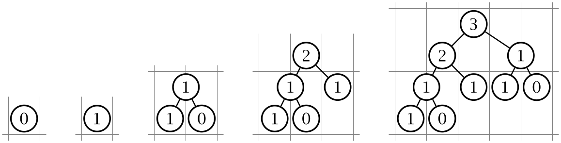
b)The first few Fibonacci trees are shown in Fig. C.5. The first two Fibonacci trees consists of a single node. The others are obtained by attaching the previous two trees to a new root node.

(-tikz- diagram)

Figure C.5 The first five Fibonacci trees.

c)As you can see in Fig. 3.6, the width of a Fibonacci tree of order \(k\) is proportional to the number of leaves in the tree. Let’s call the number of leaves of an order-\(k\) tree \(L_k\). The first two Fibonacci trees consist of just a single node, so we have

\begin{equation} L_0 = L_1 = 1 \end{equation}

In all other cases, \(L_k\) is the number of leaves in the left subtree plus the number of leaves in the right subtree. Since the left subtree is a Fibonacci tree of order \(n-1\) and the right subtree a Fibonacci tree of order \(n-2\), we have

\begin{equation} L_k = L_{k-1} + L_{k-2},\qquad \text {for $k\ge 2$}. \end{equation}

The recursive definition of \(L_k\) is therefore almost identical to the definition of the Fibonacci numbers themselves and only differ for \(k=0\). It’s not hard to see that

\begin{equation} L_k = F_{k+1}. \end{equation}

For example, the number of leaves in Fig. 3.6 is \(F_9=21+13=34\). The height of a Fibonacci tree of order \(k\) is usually simply \(k\), except for \(k=0\) where the height is 1.

d)A program for constructing the Fibonacci tree of a given order is shown in Listing C.15. The parameter bottomLeft is the coordinate of the bottom-left corner of the entire tree. If the order is 0 or 1, we place a single leaf node at bottomLeft. Otherwise, we first compute the left and rigth subtrees and then the position of the root node. The lower-left corner of the left subtree is bottomLeft and the right subtree is moved right and up to align the two subtrees at the top. The root node is placed centered above the two subtrees. The functions width() and height() compute the width and height of a Fibonacci tree using the formulas we derived in the part (c).

Listing C.15ch3 / FibonacciTree

public static double width(int order) {
    return fib(order + 1);
}

public static double height(int order) {
    return Math.max(order, 1.0);
}

public static void drawFibonacciTree(int order, Point bottomLeft) {
    if (order <= 1) {
        System.out.printf("%d at %s%n", fib(order), bottomLeft);
    } else {
        double leftWidth = width(order - 1);
        double rightWidth = width(order - 2);
        double leftHeight = height(order - 1);
        double rightHeight = height(order - 2);
        drawFibonacciTree(order - 1, bottomLeft);
        var originRight = new Point(
                bottomLeft.x() + leftWidth,
                bottomLeft.y() + leftHeight - rightHeight);
        drawFibonacciTree(order - 2, originRight);
        var rootPosition = new Point(
                bottomLeft.x() + (leftWidth + rightWidth - 1) / 2,
                bottomLeft.y() + leftHeight);
        System.out.printf("%d at %s%n", fib(order), rootPosition);
    }
}

JDK: Math, System
Point: Point()

Solution to Exercise 3.8

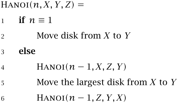
a)The key insight is that the largest disk can only be moved from A to B if the three small disks are on the rightmost peg. The four-disk problem can therefore be solved by first moving the three smallest disks from A to C, then the largest disk from A to B, and finishing by moving three disks from C to B. To transfer the smaller three-disk tower we use the same strategy recursively.

b)Suppose we want to move a tower of \(n\) disks from the peg labeled X to another peg labeled Y. The third peg labeled Z is assumed to be empty or contain only larger disks. A recursive algorithm can then be formulated as follows:

(image)

c)The recursive implementation in Listing C.16 takes four arguments: the total number of disks numDisks, the number of disks n that should be moved, and the source and destination pegs. We refer to the three pegs using the upper-case letters 'A', 'B', and 'C'. The function returns immediately if the tower is empty or source is equal to destination. Otherwise, the index of the third peg tmp is computed using the following trick:

'A' + 'B' + 'C' - destination - source

This expression uses the fact that the numerical sum of all three peg indexes is always 'A'+'B'+'C'. The index of the largest disk being transferred in each step is numDisks + 1 - n.

Listing C.16ch3 / Hanoi

public static void solveHanoiMoves(
        int numDisks, int n, char source, char destination) {
    if (n == 0 || source == destination)
        return;
    int tmp = 'A' + 'B' + 'C' - destination - source;
    solveHanoiMoves(numDisks, n - 1, source, (char) tmp);
    System.out.printf("Move disk %d from %c to %c%n",
            numDisks + 1 - n, source, destination);
    solveHanoiMoves(numDisks, n - 1, (char) tmp, destination);
}

d)Transferring a three-disk tower requires 3 moves, and for a four-disk tower it’s already \(2\cdot 7+1=15\) moves. It’s easy to prove using induction that \(2^n-1\) moves are necessary to move an \(n\)-disk tower. Moving a 64-disk tower therefore requires \(2^{64}-1\) or 18 446 744 073 709 551 615 moves. Even if the priests were able to move one disk per second, transferring the whole tower would take 585 billion years — 42 times the age of the known universe! It’s therefore quite likely that, almost no matter for how many centuries or millennia the priests have already been at work, the world will come to an end long before they are able to move the final disk.

e)The optimal way to reorganize the disks consists of five steps:

B to C, A to C, A to B, C to B, C to A.

The intermediate configurations are ABA, ACA, ACC, BCC, BCB, and BAB.

f)The problem can again be solved recursively. To transform the configuration \(x_0x_1\dots {}x_{n-1}\) into the configuration \(y_0y_1\dots {}y_{n-1}\), first move the \(n-1\) smallest disks out of the way, then move the largest disk from position \(x_0\) to position \(y_0\), and finally move the \(n-1\) smallest disks to their correct positions. More specifically, if \(z\) is the third peg that differs from both \(x_0\) and peg \(y_0\), the steps are as follows:

  • 1. Recursively move \(n-1\) disks from \(x_1 x_2\dots {}x_{n-1}\) to \(zz\dots {}z\).

  • 2. Move a single disk from \(x_0\) to \(y_0\).

  • 3. Recursively move \(n-1\) disks from \(zz\dots {}z\) to \(y_1y_2\dots {}y_{n-1}\).

As a special case, if \(x_0=y_0\), we only have to recursively transform \(x_1\dots {}x_{n-1}\) into \(y_1\dots {}y_{n-1}\). An implementation of this algorithm is shown in Listing C.17. It takes 26 steps to transform BCBAC into CCCCC.

Listing C.17ch3 / Hanoi

// Find a sequence of moves that solves the Towers of Hanoi for
// arbitrary start and end states.
public static void solveHanoiPath(String start, String end) {
    int n = start.length();
    if (n == 0)
        return;
    char x0 = start.charAt(0), y0 = end.charAt(0);
    if (x0 == y0) {
        solveHanoiPath(start.substring(1), end.substring(1));
    } else {
        char z = (char) ('A' + 'B' + 'C' - x0 - y0);
        char[] tmp = new char[n - 1];
        for (int i = 0; i < n - 1; i++)
            tmp[i] = z;
        solveHanoiPath(start.substring(1), new String(tmp));
        System.out.println("Move disk from " + x0 + " to " + y0);
        solveHanoiPath(new String(tmp), end.substring(1));
    }
}