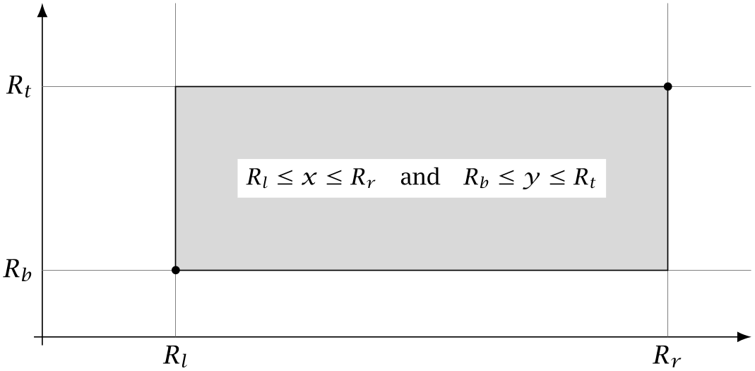
Exercise 1.4.A simple geometric shape that is useful in many applications is the axis-aligned rectangle, a rectangle whose sides are parallel to the coordinate axes. As shown in Fig. 1.6, each such a rectangle \(R\) is uniquely defined by the position of its four edges: the left and right edges
\(R_l\) and \(R_r\) and the top and bottom edges \(R_t\) and \(R_b\). The interior of such a rectangle consists of all points \((x,y)\) that satisfy
\(\seteqnumber{0}{1.}{3}\)
\begin{equation*}
R_l \le x \le R_r\qquad \text {and}\qquad R_b \le y \le R_t.
\end{equation*}
The rectangle is empty if there are no points that satisfy these relations; this is the case if either \(R_l > R_r\) or \(R_b > R_t\).
Figure 1.6 An axis-aligned rectangle.
a) Given a set of points \(\vec {p}_1,\dots , \vec {p}_n\), how do you compute the smallest axis-aligned rectangle that contains all points?. (This rectangle is also referred to as the point set’s bounding box).
b) Given two axis-aligned rectangles \(A\) and \(B\), how do you compute the smallest axis-aligned rectangle that encloses them both?
c) If two axis-aligned rectangles overlap, their intersection is also an axis-aligned rectangle. How do you compute its coordinates? The left (top) edge of the intersection must be the maximum of the two left (top) edges of the original rectangles, and
the right (bottom) edge is the minimum of the two right (bottom) edges. These expressions also handles the special case in which the two rectangles don’t overlap; in this case, the returned rectangle has a negative width or height and is therefore considered empty.
d) Listing 1.10 shows one possible way of defining a data type Rectangle for working with axis-aligned rectangles. Implement the missing methods.
public record Rectangle(Point bottomLeft, Point topRight) {
    // The width and height of the rectangle.
    public int width();
    public int height();

    // Is the rectangle empty?
    public boolean isEmpty();

    // Determine whether 'p' lies inside the rectangle.
    public boolean contains(Point p);

    // Return intersection of 'this' and 'r'.
    public Rectangle intersection(Rectangle r);

    // The smallest rectangle that includes all points in the list.
    public static Rectangle boundingBox(List<Point> points);
}
Listing 1.10 Outline of a data type for representing axis-aligned rectangles.
Variations of the Chaos Game
Exercise 1.5. A simple heuristic for computing the probabilities associated with an affine IFS is based on determinants. For a \(2\times 2\) matrix \(\vec {A}\), the determinant \(\det \vec {A}\) can be computed as follows:
\(\seteqnumber{0}{1.}{3}\)
\begin{equation*}
\det \vec {A} = \det \begin{pmatrix} a & b\\ c& d \end {pmatrix} = ac - bd.
\end{equation*}
A fundamental result from linear algebra is that a linear transformation of the form
\(\seteqnumber{0}{1.}{3}\)
\begin{equation*}
\vec {p} \mapsto \vec {A}\vec {p}=\begin{pmatrix} a & b\\ c& d \end {pmatrix}\vec {p}
\end{equation*}
scales the area of any shape by the factor \(\det \vec {A}\). In the case of the Barnsley fern, for example, the areas of the four parallelograms shown in Fig. 1.4 are proportional to the
determinants of the matrix parts of the corresponding functions. (If the determinant is negative, the transformation mirrors one of the coordinate axes; in this case, the absolute value of the determinant must be used.)
a) Compute the determinants of the four matrices that are used in the definition of the Barnsley fern. What do you observe?
b) Suggest a way to turn the values you obtain into probabilities that measure the footprint of each function.
Exercise 1.6.In the simplest version of the chaos game, which we discussed at the beginning of this chapter, the current point is always moved halfway
toward a random corner of a triangle. In this exercise we discuss a few interesting variations of this simple procedure.
The first variation is to replace the triangle with another regular polygon:
The easiest way to construct these polygons is to use polar coordinates, which specify the position of a point using its distance \(r\) from the origin and the angle \(\phi \) it makes with the \(x\)-axis, as illustrated in the left part of Fig. 1.7. Polar coordinates \((r,\phi )\) are related to the conventional Cartesian coordinates \((x,y)\) by elementary trigonometry:
\(\seteqnumber{0}{1.}{3}\)
\begin{equation}
\label {eq:polar} x = r\cos \phi ,\qquad y = r\sin \phi .
\end{equation}
Figure 1.7 (Left) Points in the plane can be specified either using Cartesian coordinates \(x\) and \(y\) or polar coordinates, which indicate the distance from the origin \(r\) and the angle \(\phi \) relative to the
\(x\) axis. (Right) Polar coordinates make it easy to specify the corners of regular polygons.
a) Extend the Point type with a factory method called polar() that constructs a Point from its polar coordinates.
b) Explain how to perform the opposite conversion, from Cartesian to polar coordinates and implement two methods Point.radius() and Point.angle() that return a Point’s polar coordinates.
Hint: to find the formula for \(\phi \), consider the ratio \(y/x\).
The right part of Fig. 1.7 illustrates how polar coordinates can be used to compute the corners of a regular \(n\)-gon that is centered on the origin. The \(n\) corners of the
polygon all have the same radius, whereas the angles are \(360^{\circ }/n\) degrees apart.
c) Implement a version of the chaos game that uses a regular \(n\)-gon as its base shape. Again, every step of the game should move the current point halfway towards a randomly chosen corners.
Another simple variation is to use a different rule for moving the current point. Instead of moving it halfway toward a corner, we can move it by a by a certain fraction \(\alpha \):
d) Experiment with different \(n\)-gons and different values of \(\alpha \) and draw the resulting point sets. For which values of \(\alpha \) does this version of the chaos game produce fractals?
Exercise 1.7.In Listing 1.4 we showed a simplified program for
drawing the point sets produced by the chaos game. To complete this program, we need to create a suitable instance of Graphics2D, which is usually either a window on the screen or a bitmap image of type BufferedImage, and we
need to scale and move the coordinates of the points so that they fit inside the window or image we are drawing into.
a) Write a program takes point sets generated by the chaos game and draws them, properly scaled, either to the screen or to a bitmap image.
b) Table 1.1 shows the parameters of four affine iterated function systems. Use the chaos game and the program developed in part (a) to generate images of the corresponding fractals.
Table 1.1
Parameters of a few affine iterated function systems!examples.
.
Name
\(a\)
\(b\)
\(c\)
\(d\)
\(t_x\)
\(t_y\)
Probability
Tree
0.01
0
0
0.45
0
0
1/4
0.42
-0.42
0.42
0.42
0
0.4
1/4
0.42
0.42
-0.42
0.42
0
0.4
1/4
-0.01
0
0
-0.45
0
0.4
1/4
Dragon curve
1/2
1/2
-1/2
1/2
0
0
1/2
-1/2
1/2
-1/2
-1/2
1
0
1/2
Letters
0
-0.2
5/8
0
1/8
0
1/9
3/8
0
0
0.2
3/16
1/2
1/9
3/8
0
0
0.2
3/16
0
1/9
0
-0.2
3/8
0
5/16
1/8
1/9
3/8
0
0
0.2
5/8
1/2
1/9
3/8
0
0
0.2
5/8
1/4
1/9
3/8
0
0
0.2
5/8
0
1/9
0
-0.2
1/8
0
3/4
3/8
1/9
0
-0.2
1/8
0
3/4
1/8
1/9
Crystal
.255
0
0
.255
.3726
.6714
0.2
.255
0
0
.255
.1146
.2232
0.15
.255
0
0
.255
.6306
.2232
0.15
.370
-.642
.642
.370
.6356
-.0061
0.75
Blending Iterated Function Systems
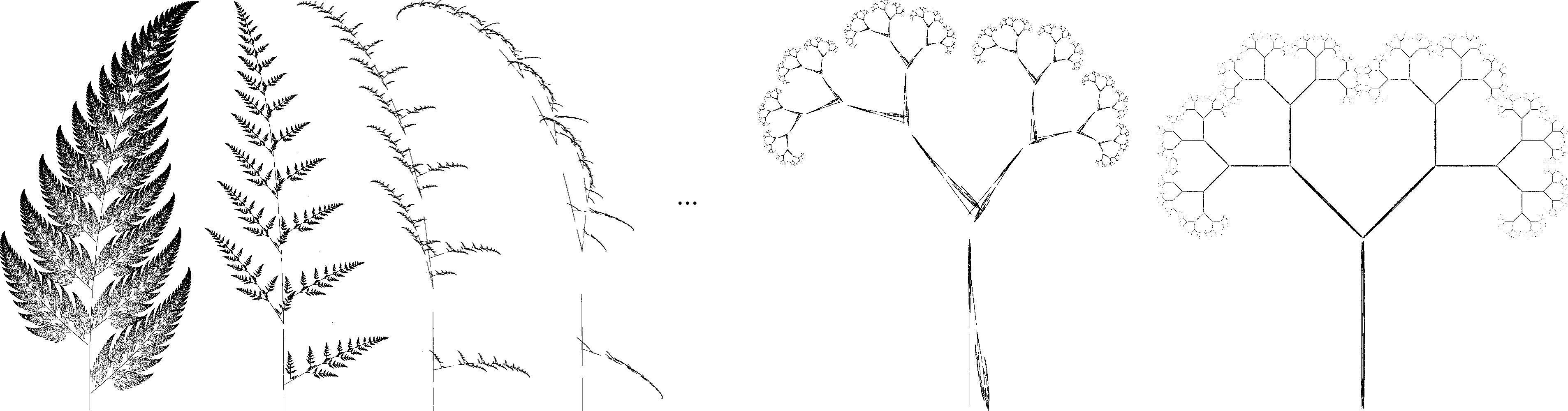
Exercise 1.8.Figure 1.8 shows a few frames from an animation that smoothly transforms the Barnsley fern on the left into the tree-shaped fractal on the right. The intermediate fractals are obtained by mixing the iterated function systems of the first and last fractal and are rendered using the standard chaos game. In this exercise we discuss how this is done.
Figure 1.8 Blending IFS fractals. The Barnsley fern on the left can be smoothly transformed into the tree-shaped fractal on the right. The intermediate fractals are obtained by interpolating the underlying
iterated function systems.
Let’s start with two arbitrary affine transformations of the form \(f(\vec {p})=\vec {F}\vec {p} + \vec {f}\) and \(g(\vec {p})=\vec {G}\vec {p}+\vec {g}\) and define a new function \(h\) that combines \(f\) and \(g\) using linear interpolation:
The parameter \(t\) is assumed to be a fixed number between 0 and 1. This new function is equal to \(f\) for \(t=0\), it is equal to \(g\) for \(t=1\), and it is a mixture of the two for every other value of \(t\).
a) Show that \(h\) is also an affine transformation and can be written as
\(\seteqnumber{0}{1.}{4}\)
\begin{align}
\label {eq:blendaffine} h(\vec {p}; t) = \lerp (\vec {F}, \vec {G}, t)\vec {p} + \lerp (\vec {f}, \vec {g},t)
\end{align}
Here, the notation \(\lerp (\vec {F}, \vec {G}, t)\) stands for the interpolation of the two matrices \(\vec {F}\) and \(\vec {G}\), which is obtained by interpolating its coefficients.
Not only can we blend individual affine transformations, we can also blend systems of affine transformations. Assume that \(F=(f_1, \dots , f_n)\) and \(G=(g_1, \dots , g_n)\) are two iterated function systems of the same size \(n\). We can now define a blended function system
\(H_t=(h_1,\dots ,h_n)\) linearly interpolating each pair of functions:
As we saw in part (a), each \(h_k\) is an affine transformation, so the system \(H\) is another affine IFS that can be rendered using the chaos game of this chapter. The parameter \(t\) indicates the time that has passed since the start of the animation: We start with the original function
system \(F=H_0\) at \(t=0\) and end with the target function system \(G=H_1\) at \(t=1\). For intermediate values of \(t\), the fractals generated by \(H_t\) are a mixture of those generated by \(F\) and \(G\).
b) Write a program that uses Eq. (1.6) to generate animations of iterated function systems similar to the one shown in Fig. 1.8. (Refer to Table 1.1 for the parameters of fractals you can use for testing.) How do you blend the tables of probabilities and how do you handle the case where the two function
systems don’t contain the same number of functions?